Maximum Flow
From Computability, Complexity & Algorithms — Charles Brubaker and Lance Fortnow
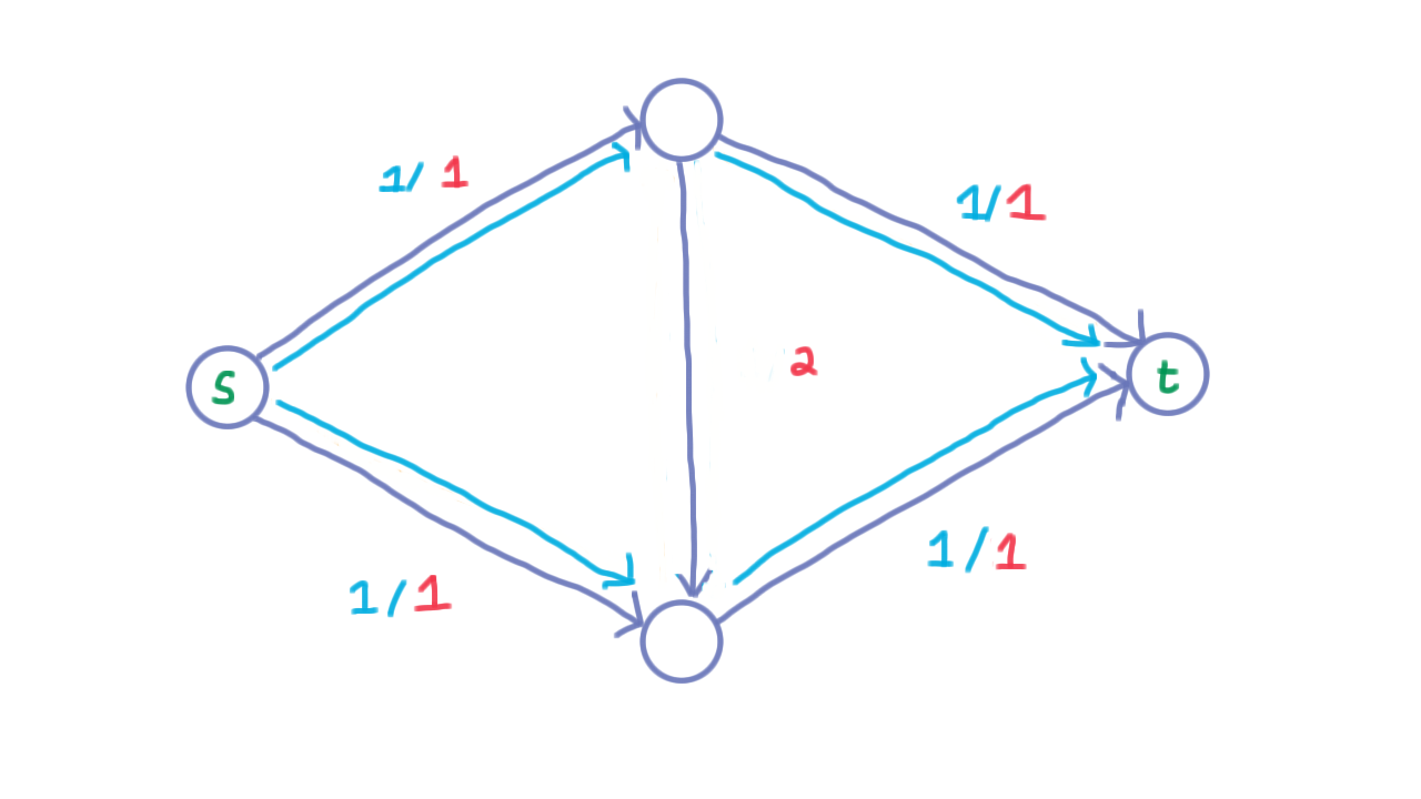
Flow Networks
A flow network is a directed graph \(G = (V, E)\) with:
A source vertex \(s\) and a sink vertex \(t\).
A capacity function \(c : E \to \mathbb{R}_{\geq 0}\).
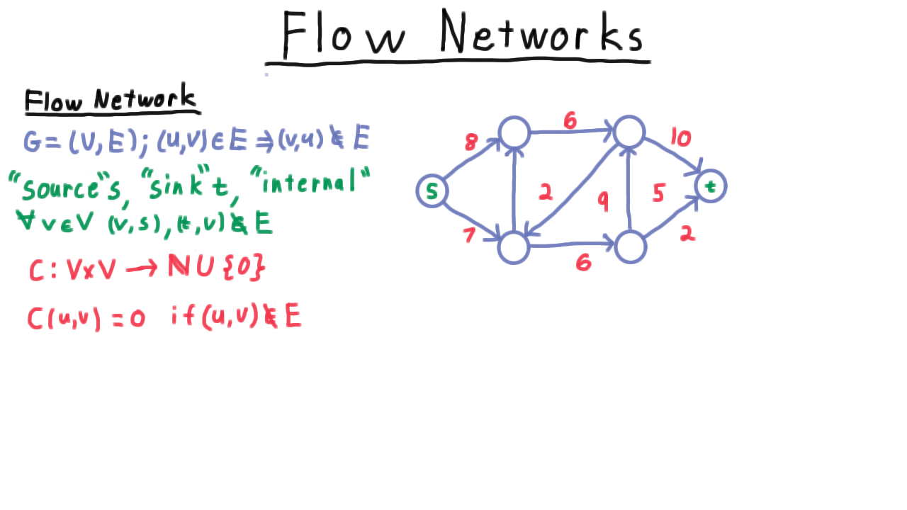
Example flow network with source, sink, and capacity labels on edges.
A flow \(f : E \to \mathbb{R}_{\geq 0}\) must satisfy:
Capacity constraint: \(0 \leq f(u,v) \leq c(u,v)\) for all edges.
Flow conservation: for every internal vertex \(u \notin \{s, t\}\):
\[\sum_{v} f(v, u) = \sum_{v} f(u, v)\]Anti-symmetry / single direction: at most one direction carries flow between any pair.
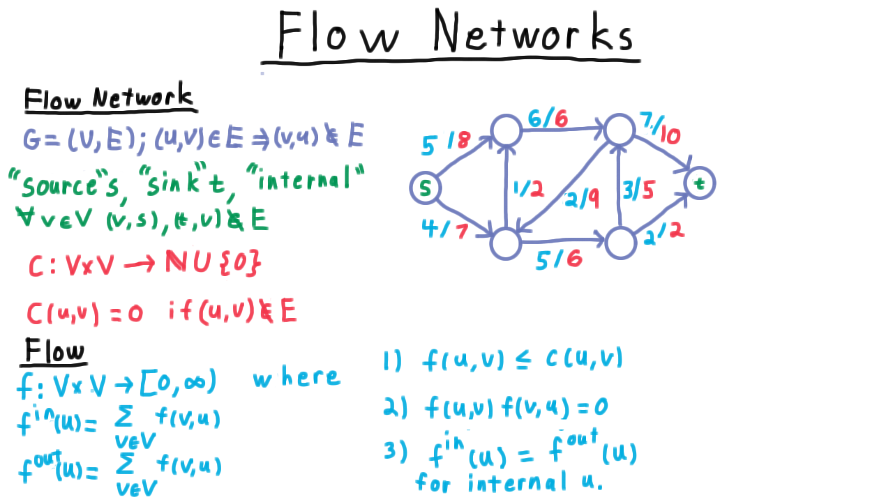
Flow conservation illustrated at an internal vertex.
The value of flow \(f\) is the total flow leaving \(s\):
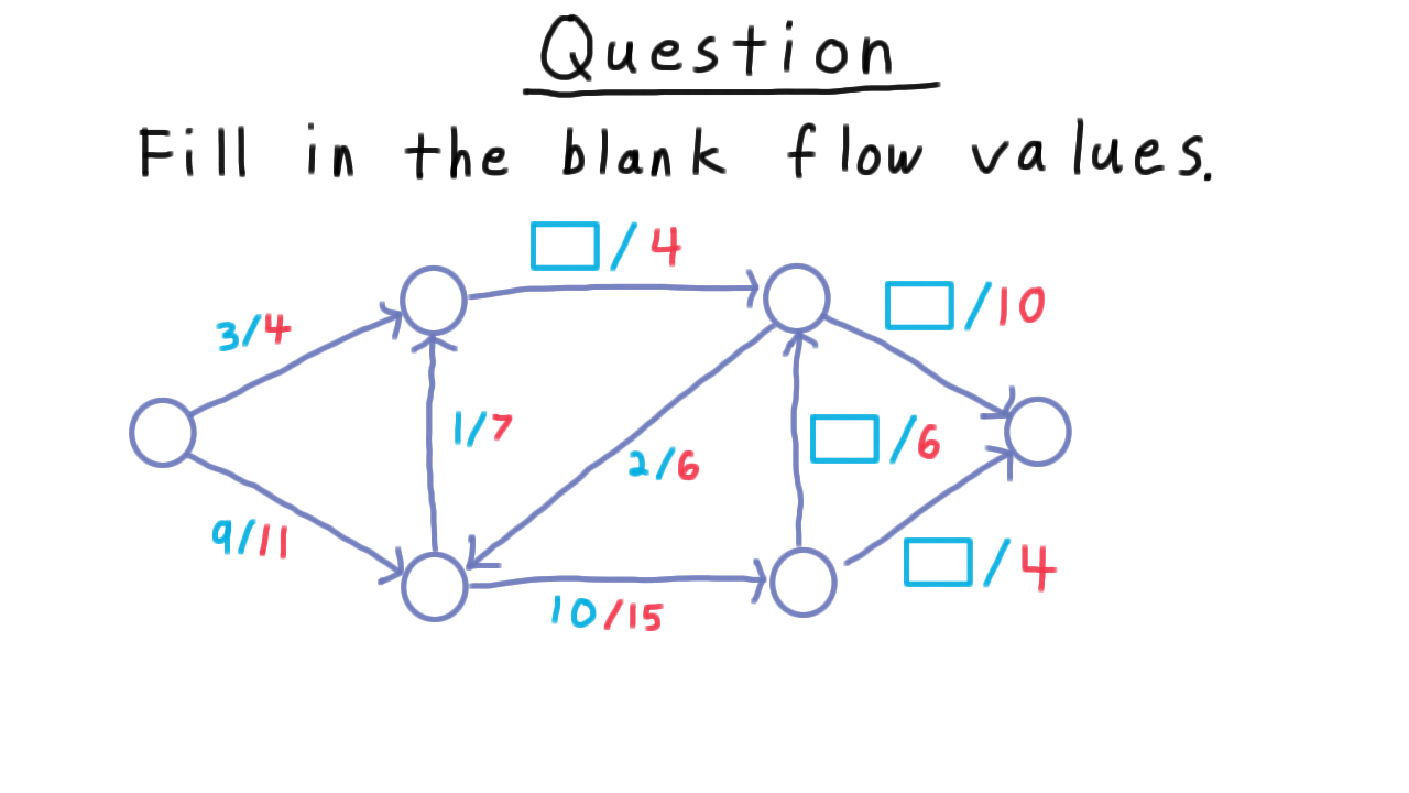
Quiz: Calculate the missing flow values on a given network.
Network Modelling Tricks
Rational capacities: Scale all capacities to integers; the algorithm still terminates.
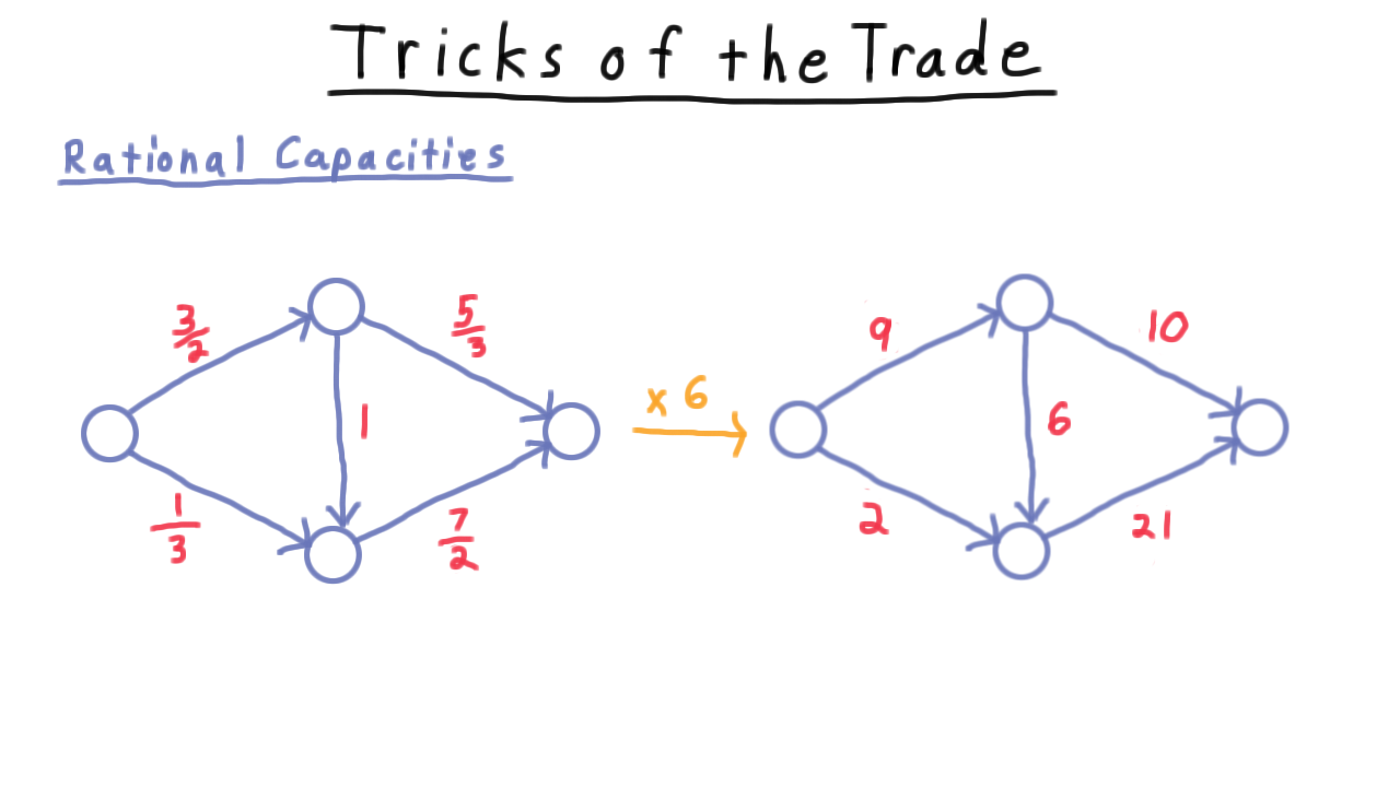
Handling rational capacities by scaling to integers.
Anti-parallel edges: Replace \((u,v)\) and \((v,u)\) with an auxiliary vertex.
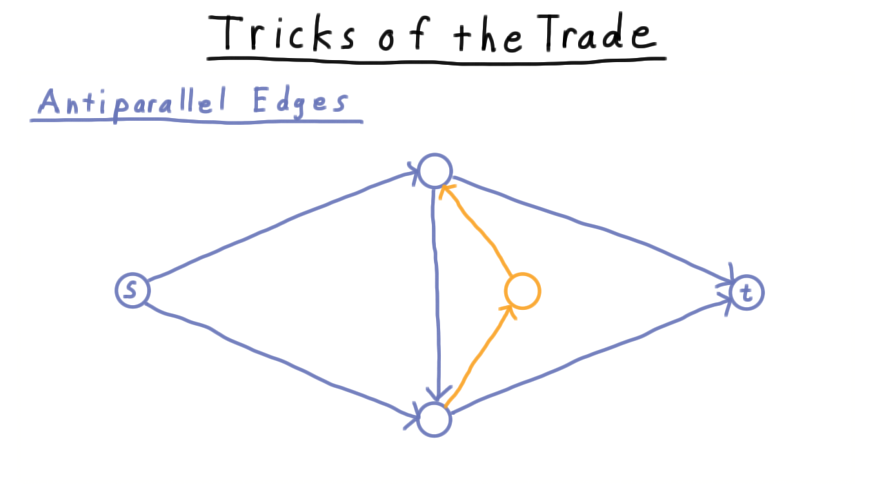
Converting anti-parallel edges using an intermediate vertex.
Multiple sources/sinks: Add a super-source \(s'\) with infinite-capacity edges to each source, and a super-sink \(t'\) from each sink.
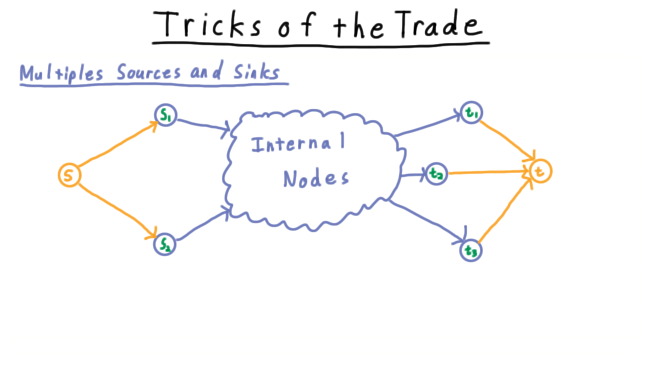
Super-source/super-sink construction for multi-commodity networks.
Ford-Fulkerson Method
Idea: Repeatedly find a path from \(s\) to \(t\) in the residual graph and push more flow along it.
Augmenting Flow
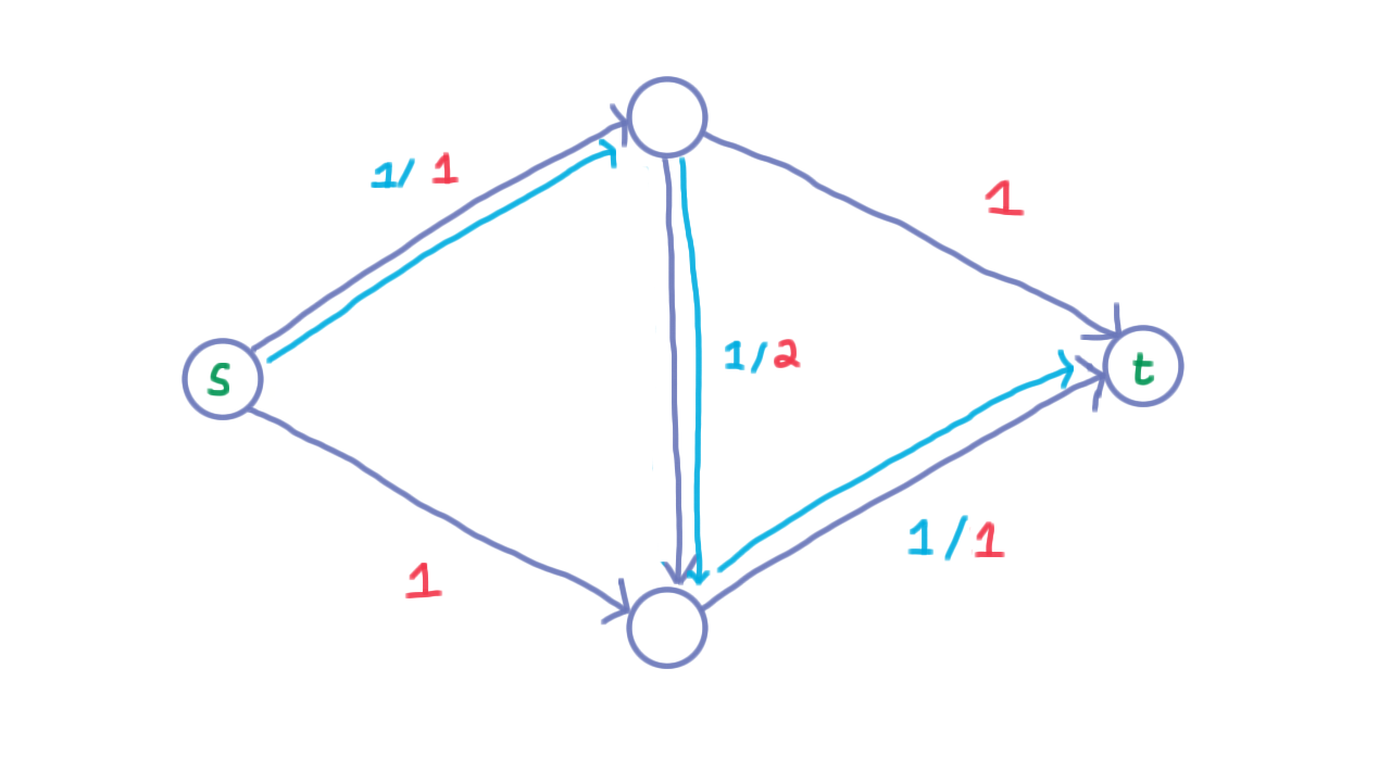
Starting flow configuration.
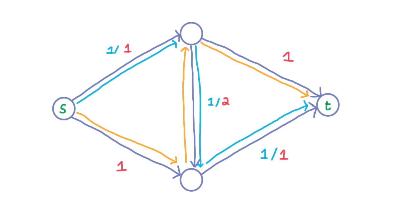
Augmenting flow (orange) added to increase the total flow value.
Result after combining initial and augmenting flows.
Residual Graph
For each edge \((u,v)\) with capacity \(c(u,v)\) and flow \(f(u,v)\), define the residual capacity:
The residual graph \(G_f\) contains all edges with positive residual capacity.
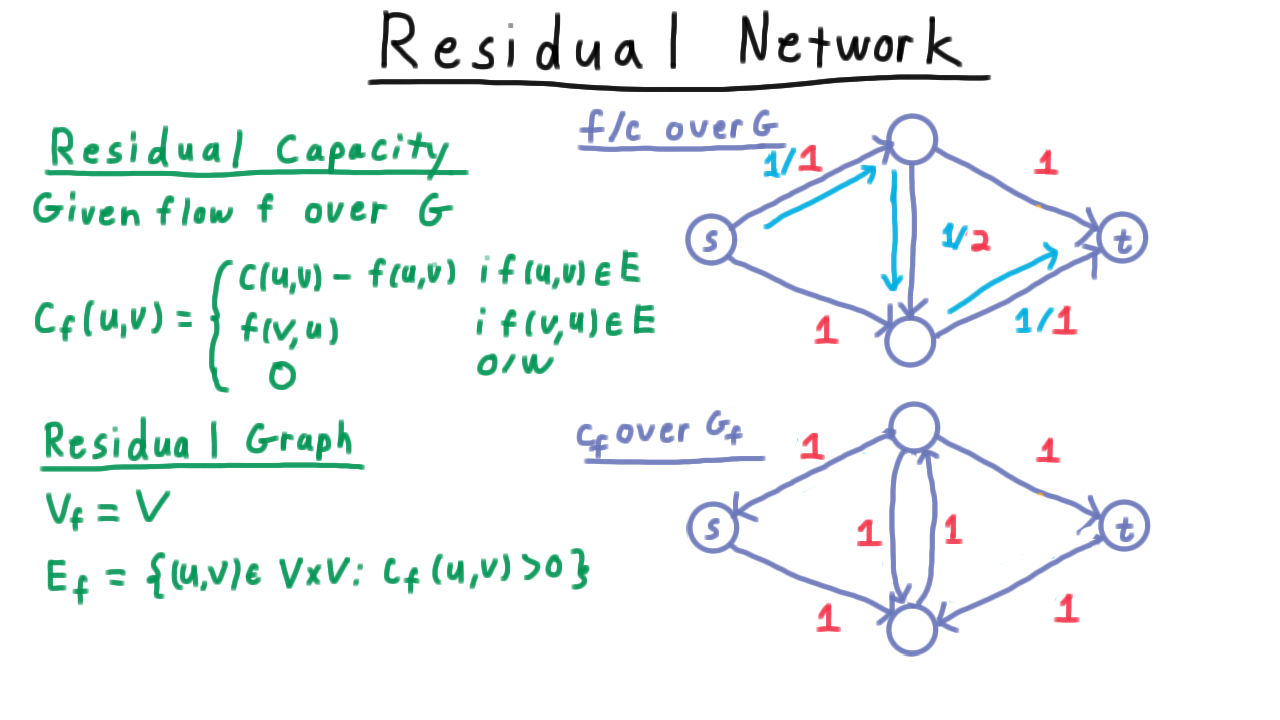
Residual capacity defined for forward and backward edges.
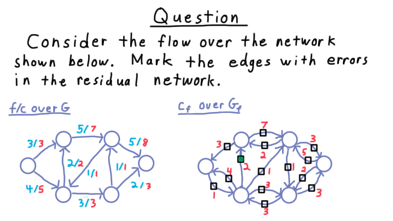
Quiz: Identify errors in a given residual network diagram.
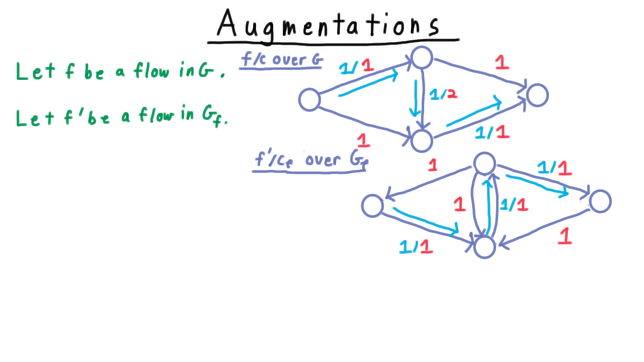
Example: augmenting flows and combining them in the residual network.
Ford-Fulkerson Algorithm
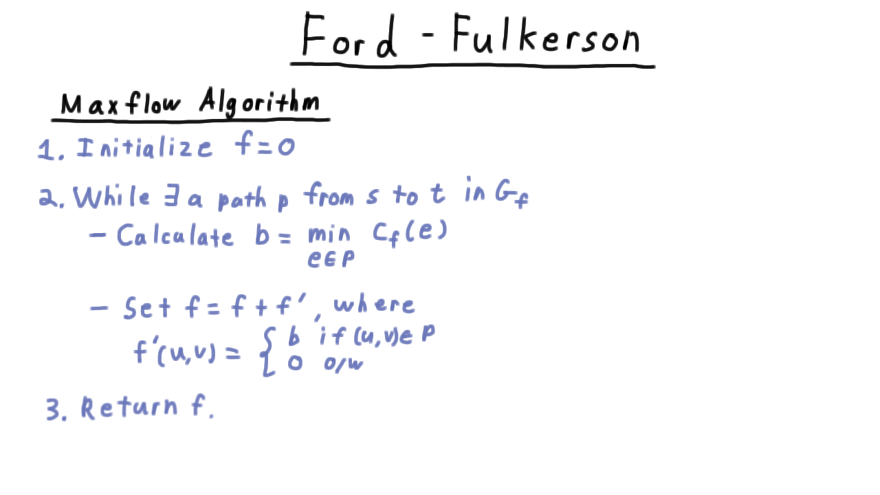
Ford-Fulkerson pseudocode.
f ← 0 (zero flow)
while ∃ augmenting path p in G_f (s → t):
    push flow along p (bottleneck capacity)
    update G_f
return f
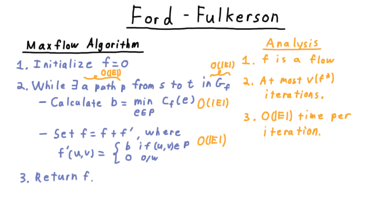
Analysis: each augmentation increases \(|f|\) by at least 1 (integer capacities), so at most \(|f^*|\) iterations, each \(O(E)\) → total \(O(E \cdot |f^*|)\).
Limitation: With poor path selection, this can be exponential in the capacity values.
Max-Flow Min-Cut Theorem
An \(s\)-\(t\) cut partitions \(V\) into sets \(A \ni s\) and \(B \ni t\). Its capacity is:
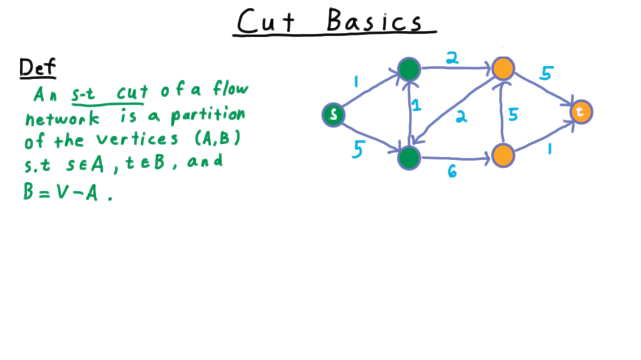
Example \(s\)-\(t\) cut — green vertices in \(A\), orange in \(B\).
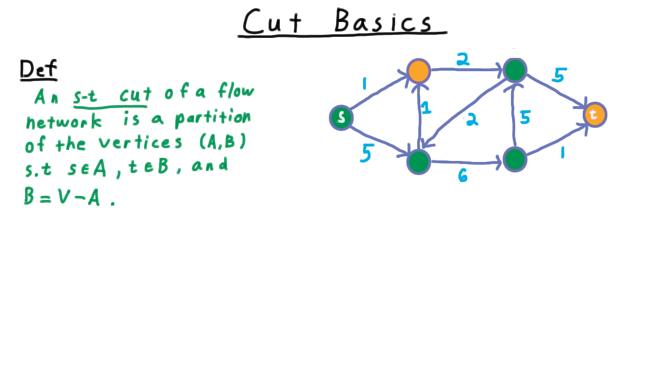
Alternative \(s\)-\(t\) cut showing a different partition.
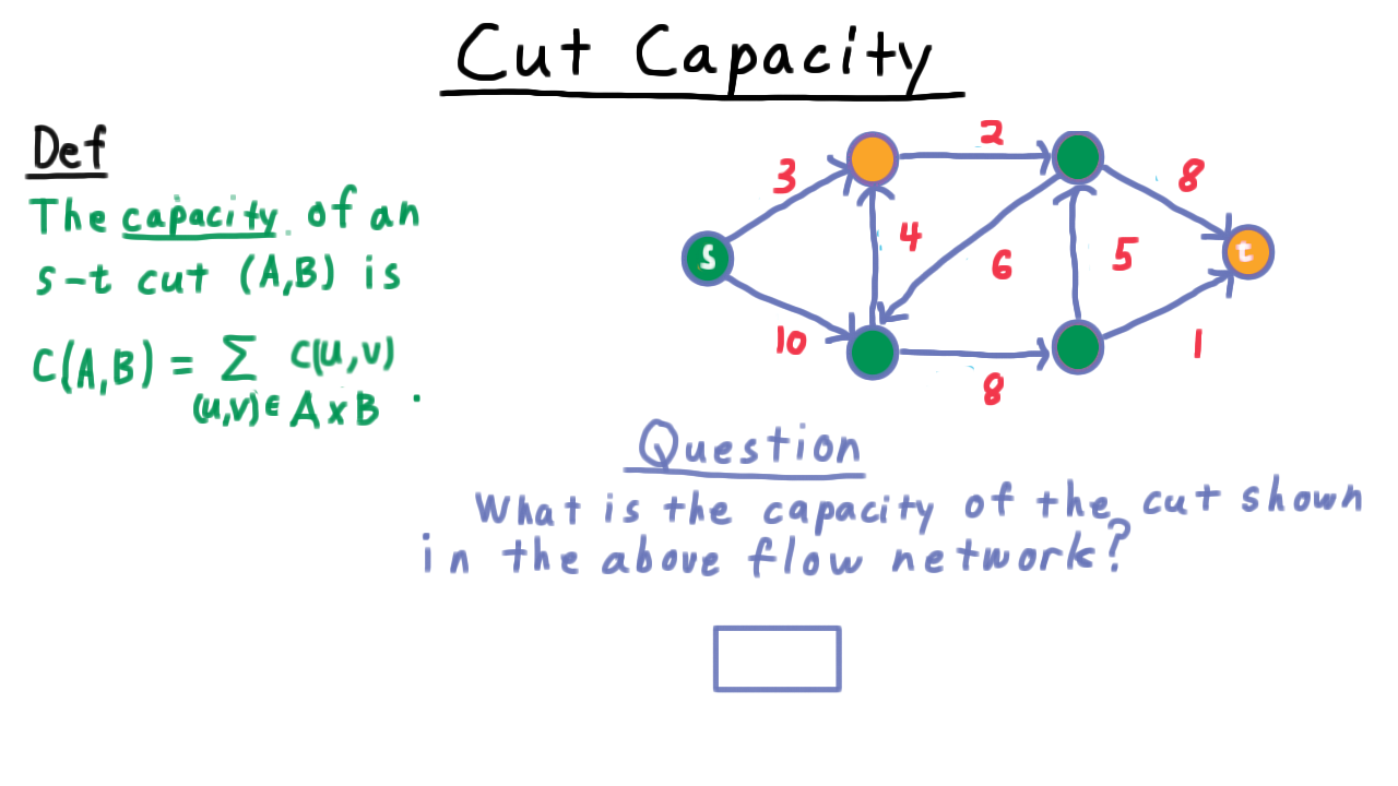
Quiz: Calculate the capacity of a given cut.
Key inequality: For any flow \(f\) and any \(s\)-\(t\) cut \((A,B)\):
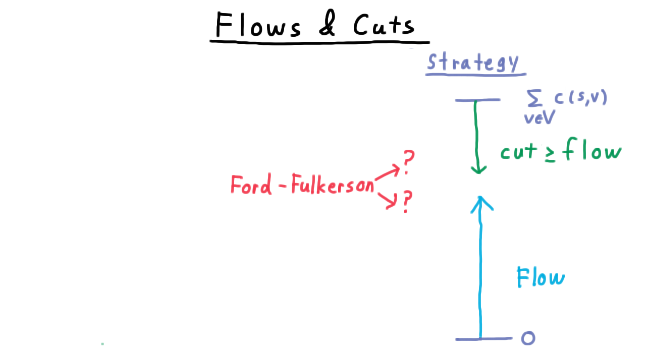
Flow value is bounded above by every cut capacity — will the bounds meet?
Strategy: show equivalence of max flow, no augmenting path, and min cut.
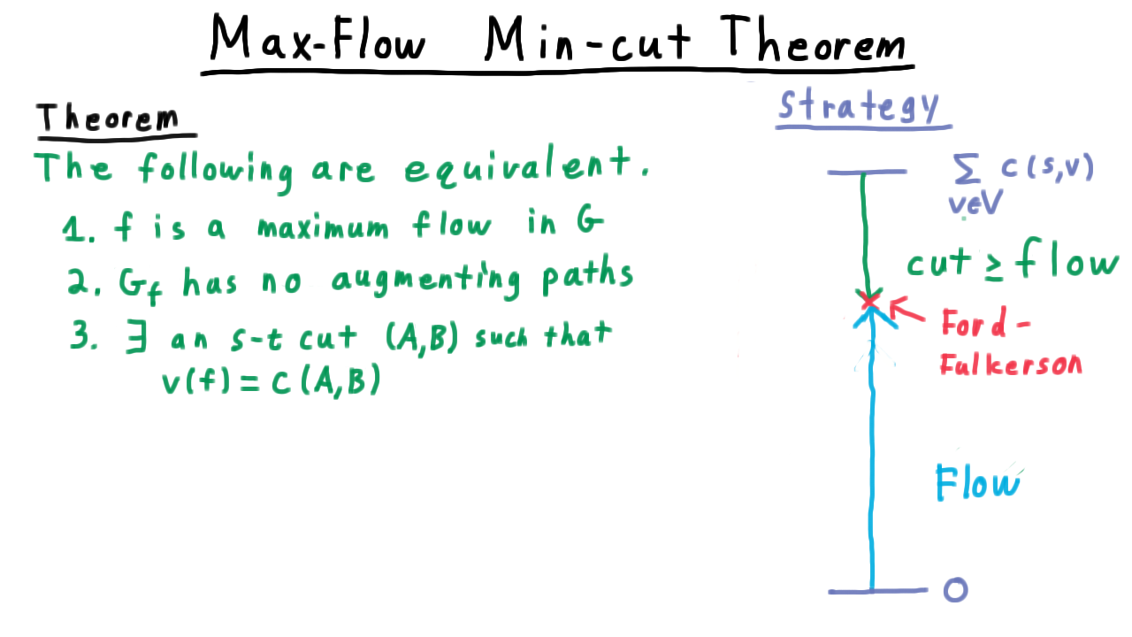
Theorem (Max-Flow Min-Cut): The following are equivalent:
\(f\) is a maximum flow.
The residual graph \(G_f\) has no \(s\)-\(t\) augmenting path.
There exists an \(s\)-\(t\) cut \((A^*, B^*)\) with \(c(A^*, B^*) = |f|\).
Proof Sketch
Define \(A^*\) as all vertices reachable from \(s\) in \(G_f\) when no augmenting path exists:
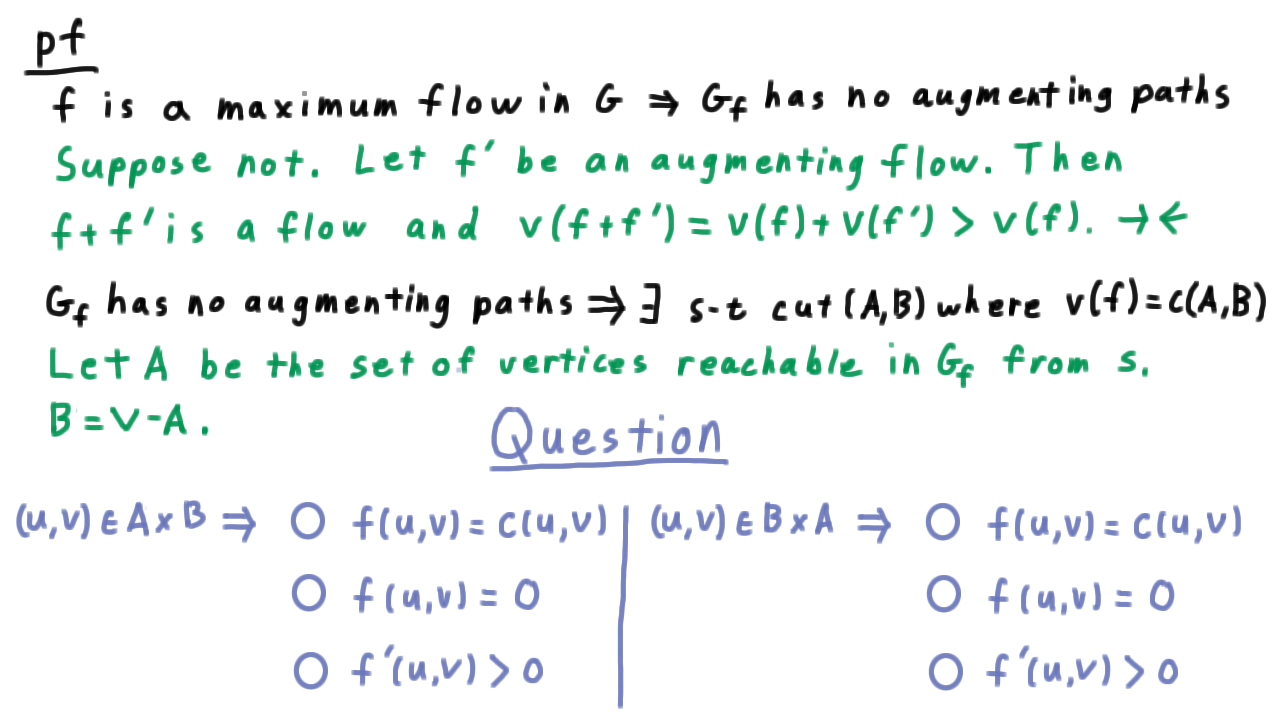
Quiz: Determine flow properties across the reachable set.
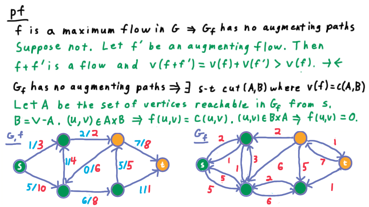
Reachable set in \(G_f\) defines a cut saturating all forward edges and cancelling all backward edges, giving \(|f| = c(A^*, B^*)\).
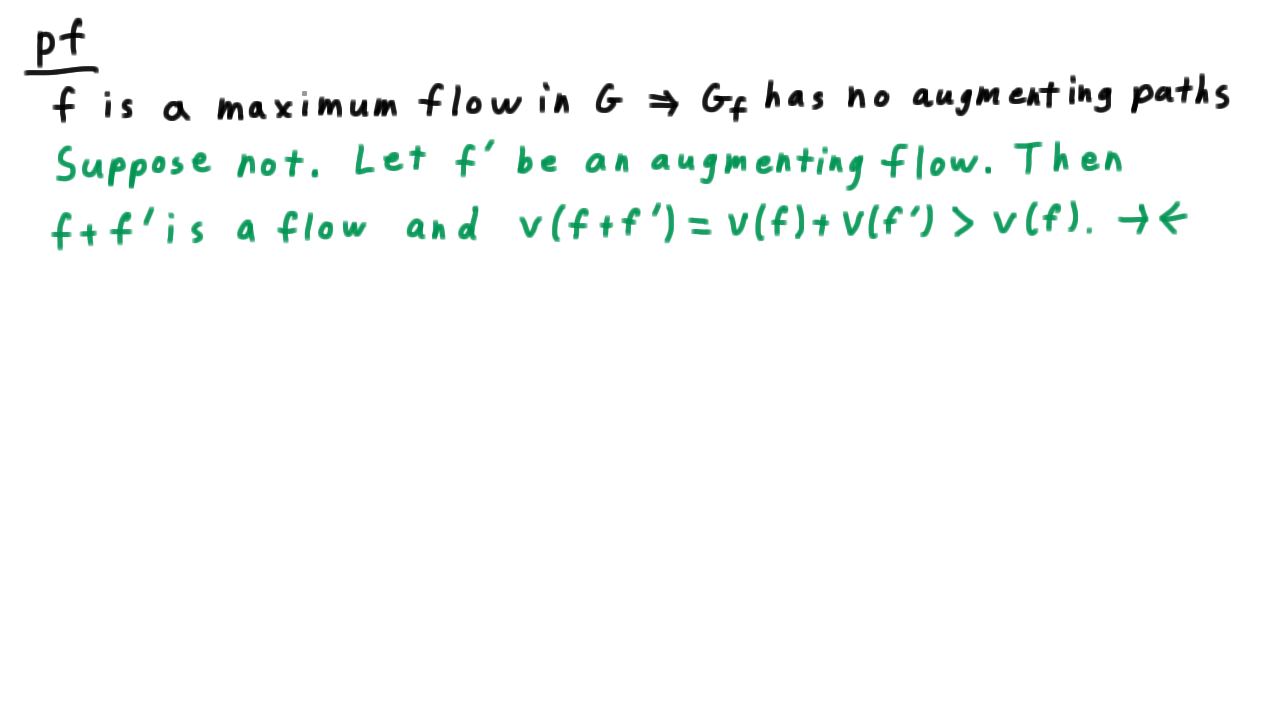
Complete proof diagram for the Max-Flow Min-Cut theorem.
Conclusion: Ford-Fulkerson terminates with a maximum flow.
Improved Algorithms
Bad Augmentation Paths
Naive path selection (e.g., DFS) can alternate between two paths and take \(O(C)\) iterations for maximum flow \(C\).
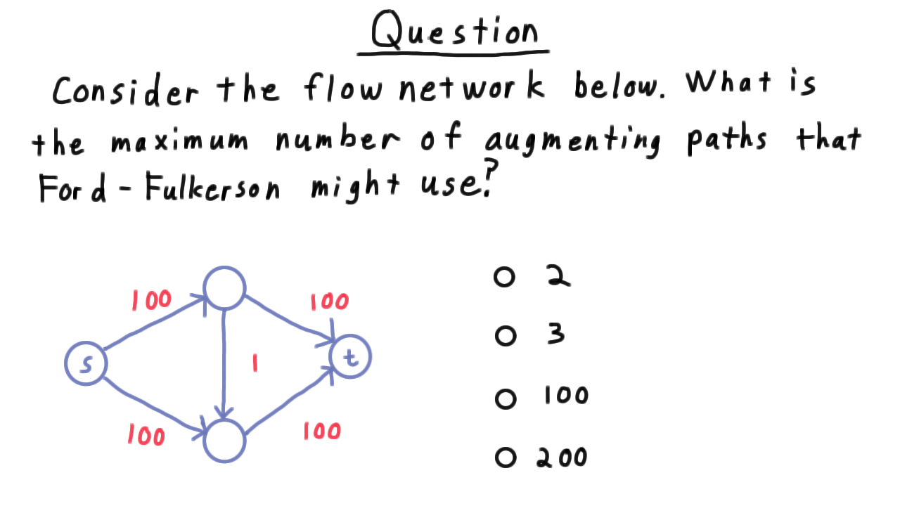
Adversarial example where poor path selection causes \(O(C)\) augmentations.
Scaling Algorithm
Prioritise augmenting paths with large bottleneck capacity using a threshold \(\Delta\):
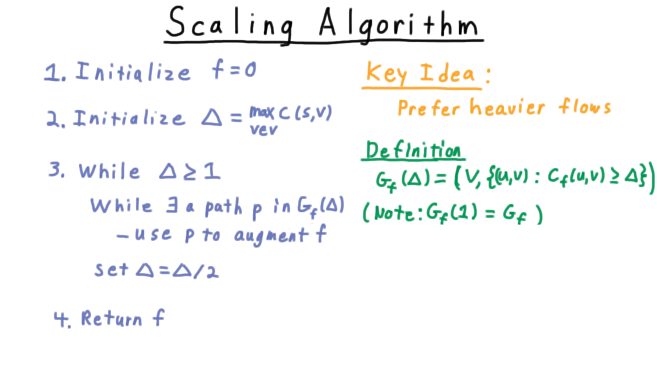
Scaling algorithm pseudocode — only use paths with bottleneck \(\geq \Delta\).
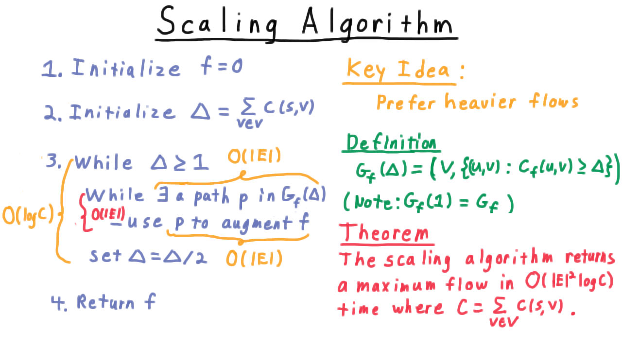
Theorem: Scaling algorithm runs in \(O(E^2 \log C)\) time.
Each scaling phase (halving \(\Delta\)) has at most \(O(E)\) augmentations, and there are \(O(\log C)\) phases.
Edmonds-Karp Algorithm
Use BFS (shortest path in terms of number of edges) to select augmenting paths:
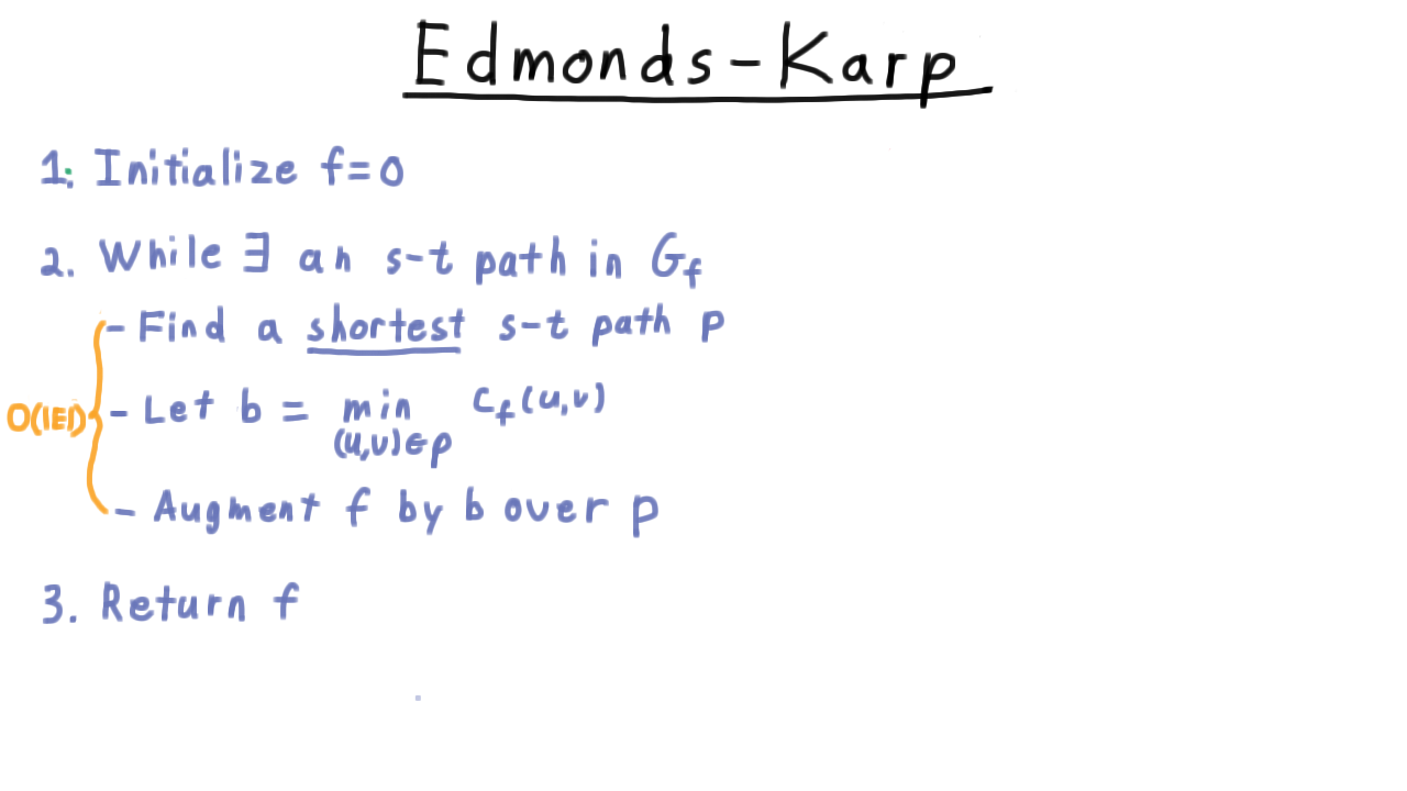
Edmonds-Karp pseudocode — Ford-Fulkerson with BFS path selection.
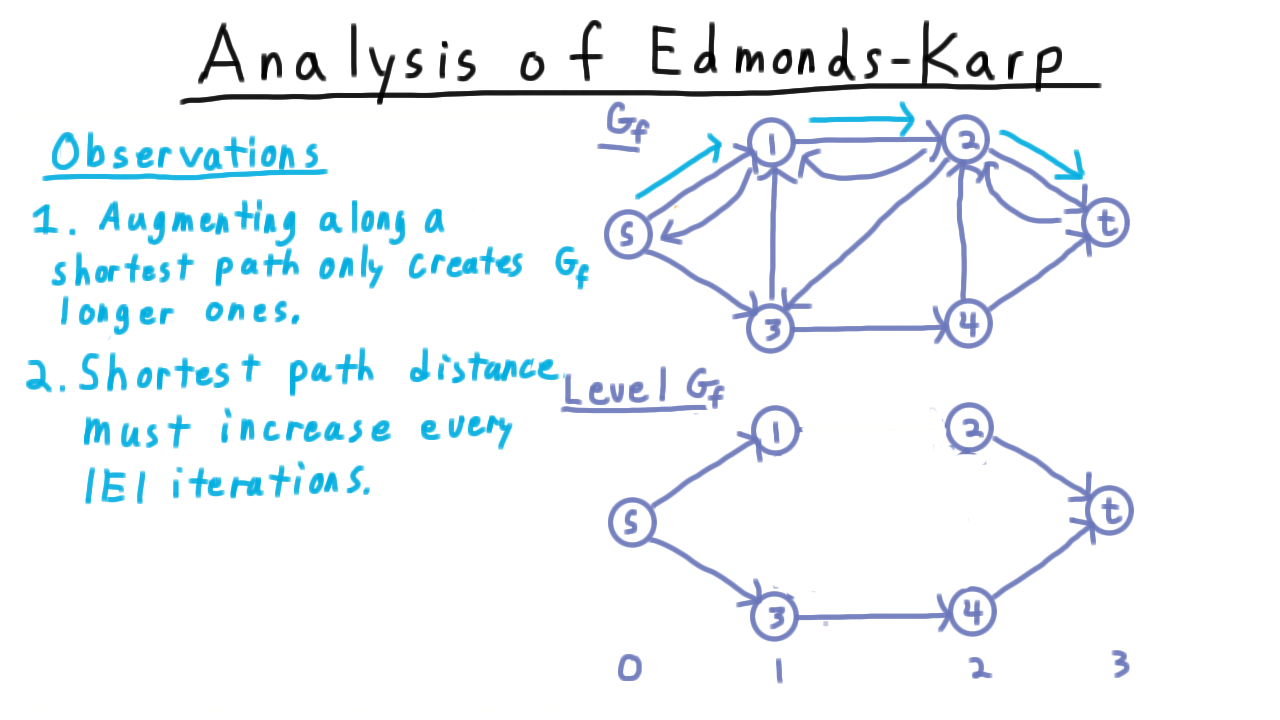
Theorem: Edmonds-Karp runs in \(O(VE^2)\) time.
Key argument: the shortest augmenting path length is non-decreasing, and each edge can be saturated at most \(O(V)\) times before the shortest path through it grows.
Dinic’s Algorithm
Build a level graph (BFS layers from \(s\)), then find a blocking flow (saturating all \(s\)-\(t\) paths in the level graph) before rebuilding:
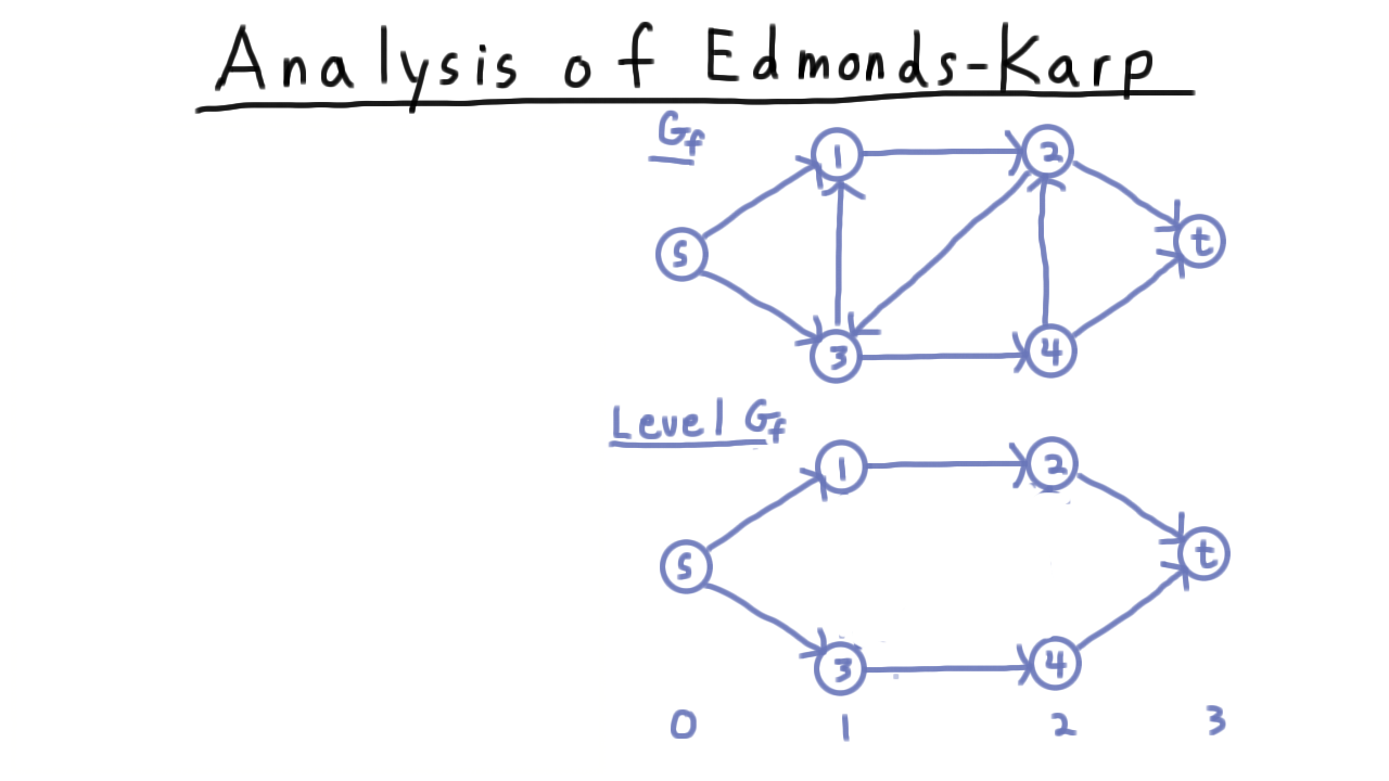
Level graph constructed by BFS layers from the source.
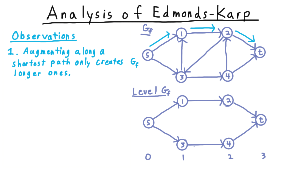
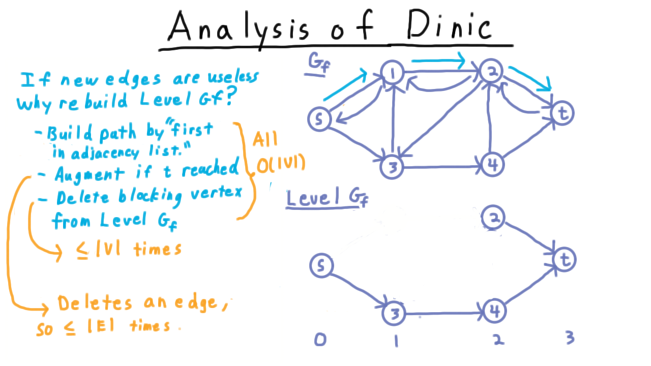
After augmentation, only backward edges are added to the level graph — no new forward shortcuts are created.
Each augmentation saturates at least one edge, bounding work per phase.
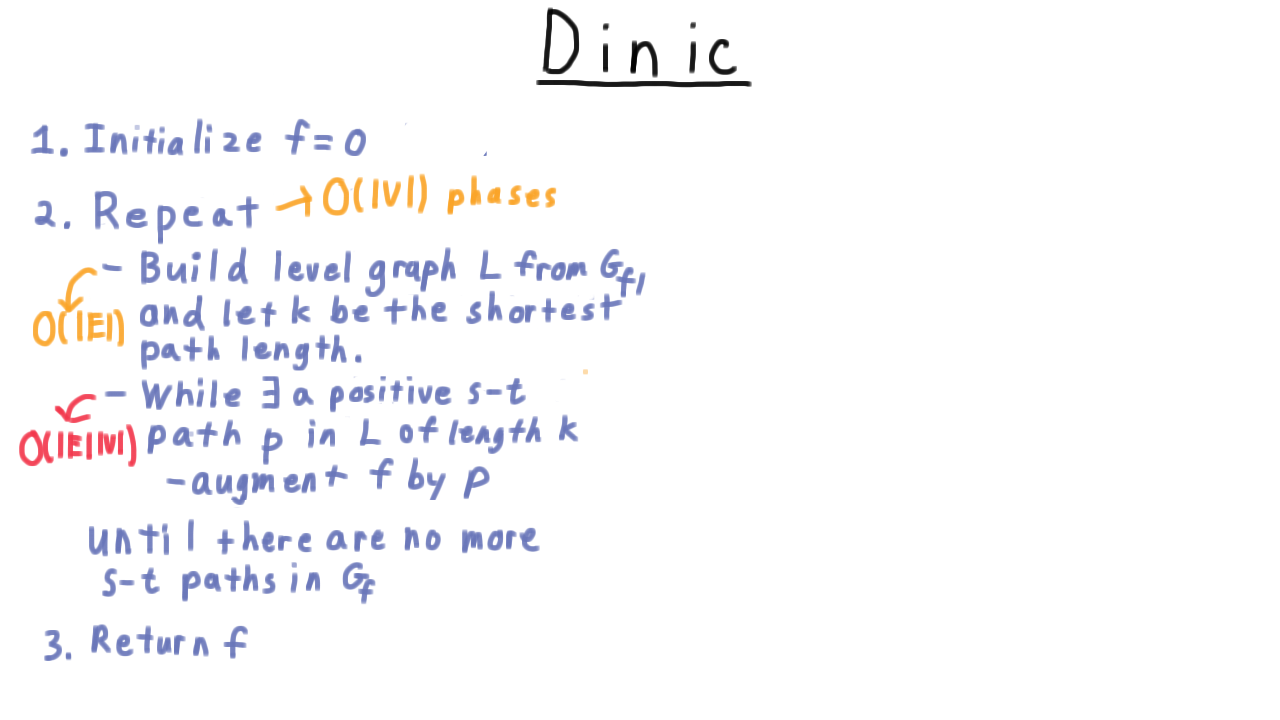
Dinic’s algorithm pseudocode with level-graph phases.
Theorem: Dinic’s algorithm runs in \(O(V^2 E)\) time.
Each phase takes \(O(VE)\) (DFS blocking flow with dead-end elimination) and there are at most \(O(V)\) phases (shortest path length grows each phase).
Complexity Summary
Algorithm |
Time Complexity |
Notes |
|---|---|---|
Ford-Fulkerson |
\(O(E \cdot |f^*|)\) |
Pseudo-polynomial; depends on max flow value |
Scaling |
\(O(E^2 \log C)\) |
\(C\) = max capacity |
Edmonds-Karp |
\(O(VE^2)\) |
Strongly polynomial |
Dinic’s |
\(O(V^2 E)\) |
Strongly polynomial; faster in practice |
Key Formulas
Residual capacity:
Flow conservation:
Weak duality (flow \(\leq\) cut):
Max-flow min-cut:
Further Reading
Bipartite matching as max flow (unit capacities)
Project selection / closure problems
Gomory-Hu trees for all-pairs max flow
Push-relabel algorithms: \(O(V^2 \sqrt{E})\)