Randomized Algorithms
From Computability, Complexity & Algorithms — Charles Brubaker and Lance Fortnow
Introduction
Randomization is a fundamental algorithmic tool. Rather than always making the same deterministic choices, randomized algorithms flip coins — and often achieve better expected performance or simpler analysis than their deterministic counterparts.
Polynomial Identity Testing
Problem: Given two polynomial representations \(A\) and \(B\) (each of degree \(\leq d\)), determine whether \(A \equiv B\).
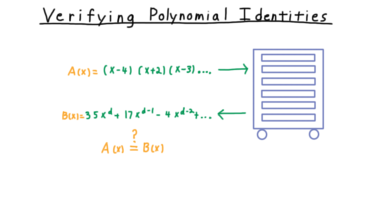
Polynomial identity testing: evaluate both polynomials at a random point.
Randomized algorithm:
Pick a random integer \(r\) uniformly from \(\{1, \ldots, 100d\}\).
Evaluate \(A(r)\) and \(B(r)\).
If \(A(r) = B(r)\), declare equal; otherwise declare unequal.
Why it works — Fundamental Theorem of Algebra:
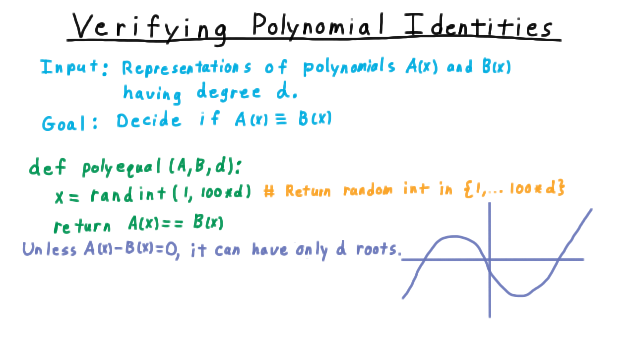
A non-zero polynomial of degree \(d\) has at most \(d\) roots.
If \(A \not\equiv B\), then \(A - B\) is a non-zero polynomial of degree \(\leq d\), so it has at most \(d\) roots. The probability of a false positive is:
Discrete Probability
A discrete probability space consists of:
Sample space \(\Omega\) — a finite or countably infinite set of outcomes.
Probability function \(\Pr : 2^\Omega \to [0,1]\) satisfying:
\[\Pr(E) \geq 0, \quad \Pr(\Omega) = 1, \quad \Pr\!\left(\bigcup_i E_i\right) = \sum_i \Pr(E_i) \text{ (disjoint events)}\]
For uniform distributions: \(\Pr(S) = |S| / |\Omega|\).
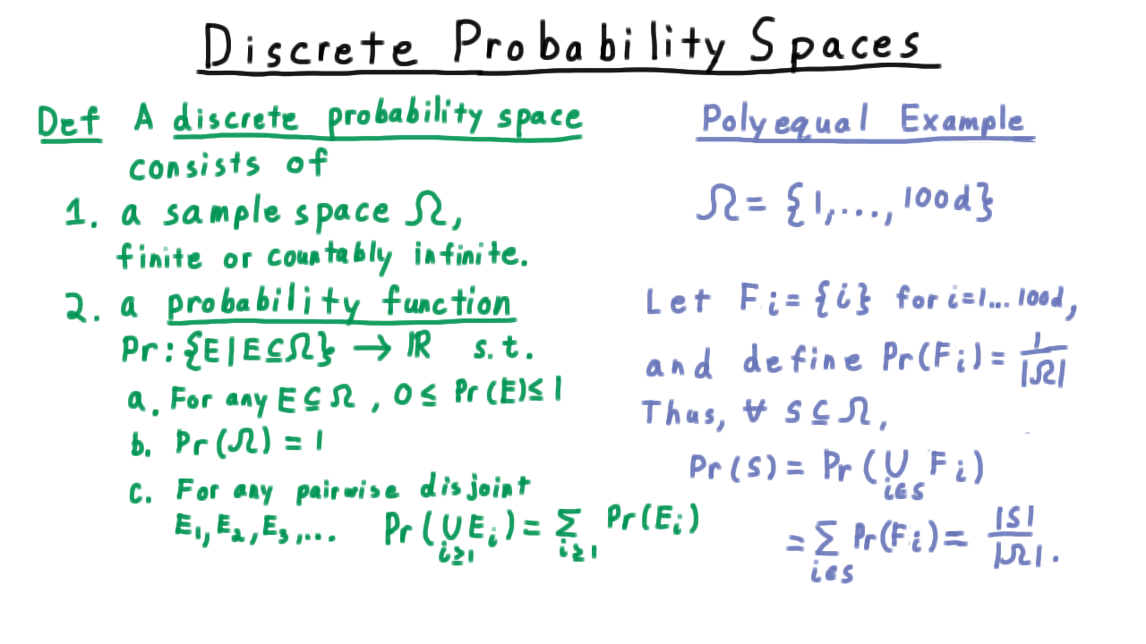
Formal definition of a discrete probability space.
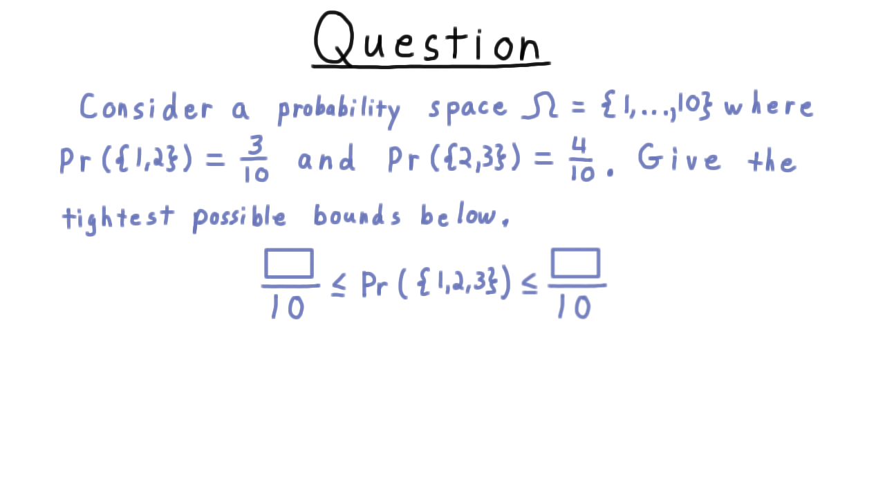
Quiz: Bound the probability of an event in a given sample space.
Repeated Trials
When running an algorithm \(k\) times independently, the probability that at least one trial succeeds (given per-trial success probability \(p\)) is:
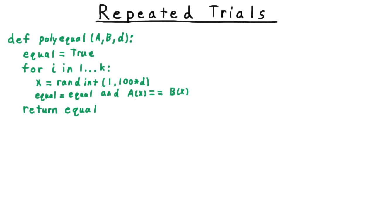
Repeated trials algorithm pseudocode.
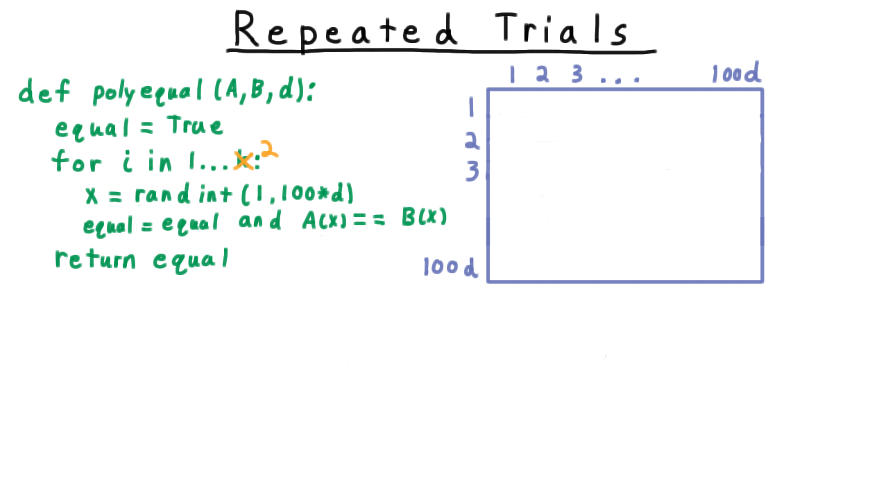
Two-dimensional sample space for two independent trials.
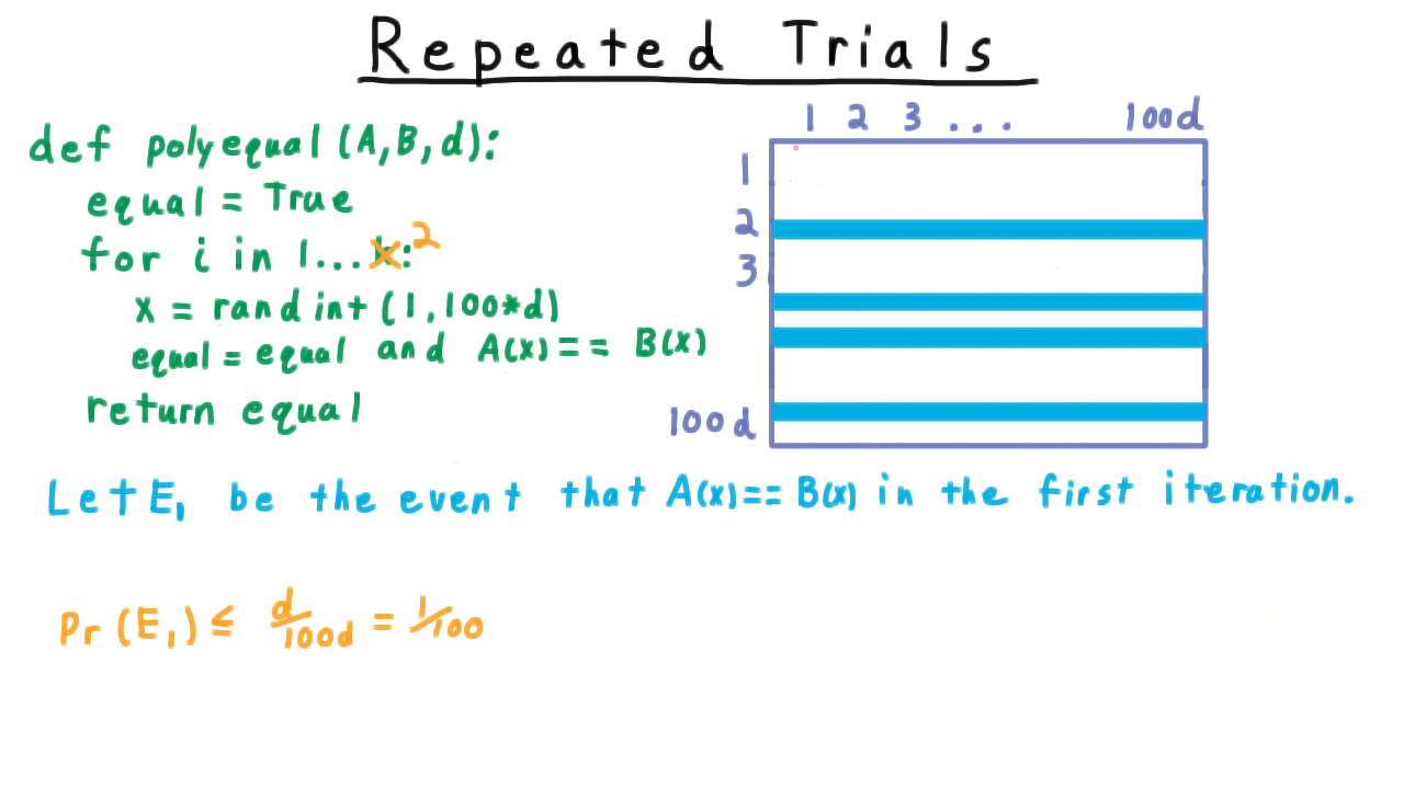
Event \(E_1\) as rows in the sample space grid.
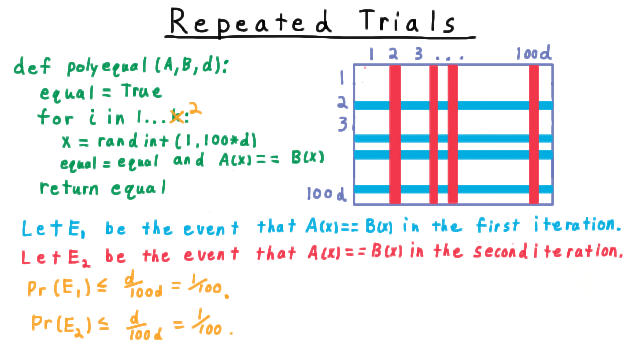
Event \(E_2\) as columns in the sample space grid.
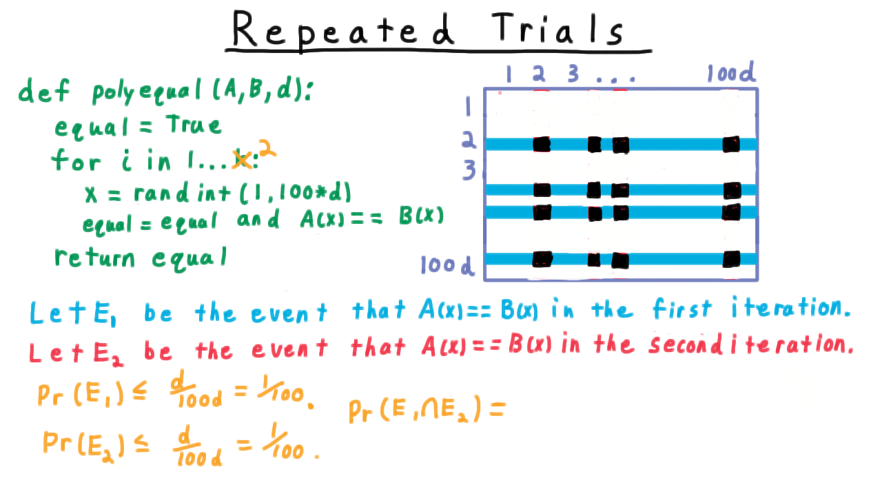
Intersection \(E_1 \cap E_2\) for independent events.
Conditional Probability and Independence
Conditional probability:
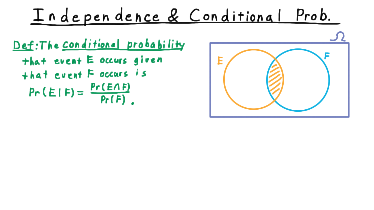
Venn diagram illustration of conditional probability.
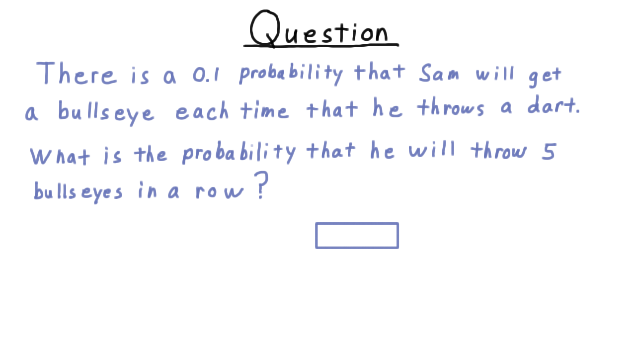
Quiz: Dart-throwing probability exercise using conditional probability.
Independence: Events \(E\) and \(F\) are independent if:
Monte Carlo vs. Las Vegas Algorithms
Monte Carlo algorithms may return incorrect answers but with bounded error probability:
One-sided error: errors only on one type of input (e.g., declaring unequal polynomials equal, never vice versa).
Two-sided error: errors possible on either type of input.
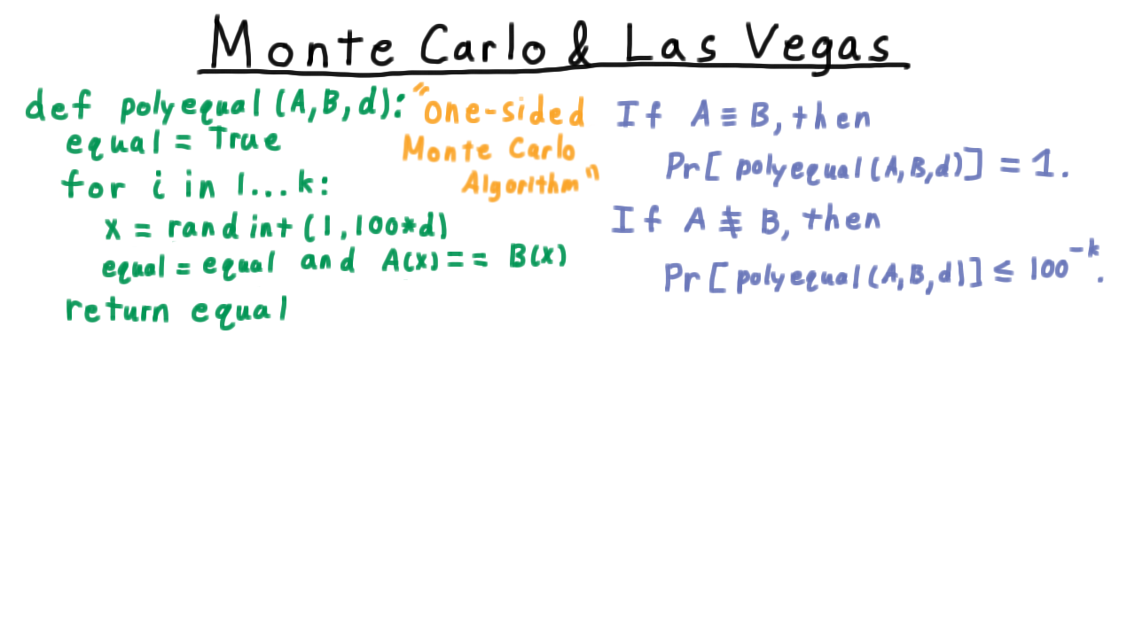
One-sided Monte Carlo: never wrong when polynomials are truly equal.
Las Vegas algorithms are always correct; randomness only affects running time.
Example: Polynomial identity testing can be made Las Vegas by sampling without replacement from \(\{1, \ldots, 100d\}\). After choosing \(d+1\) distinct points, at least one must be a non-root if \(A \not\equiv B\).
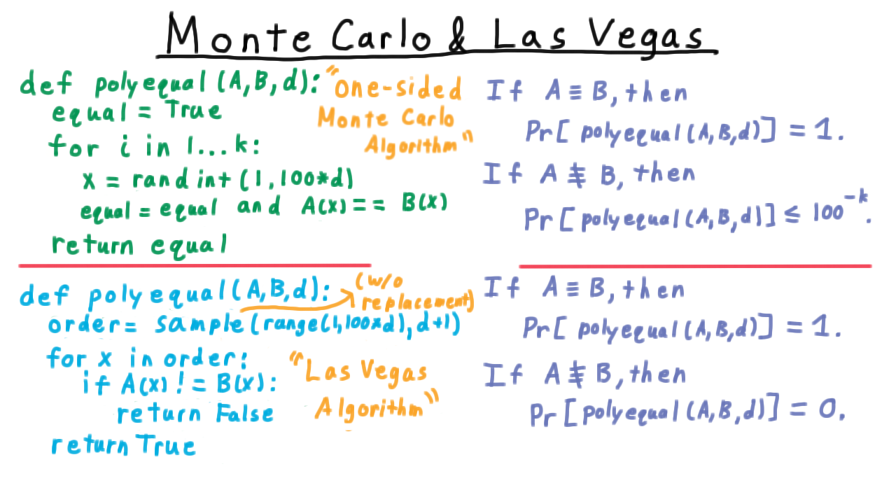
Las Vegas variant: sampling without replacement guarantees correctness.
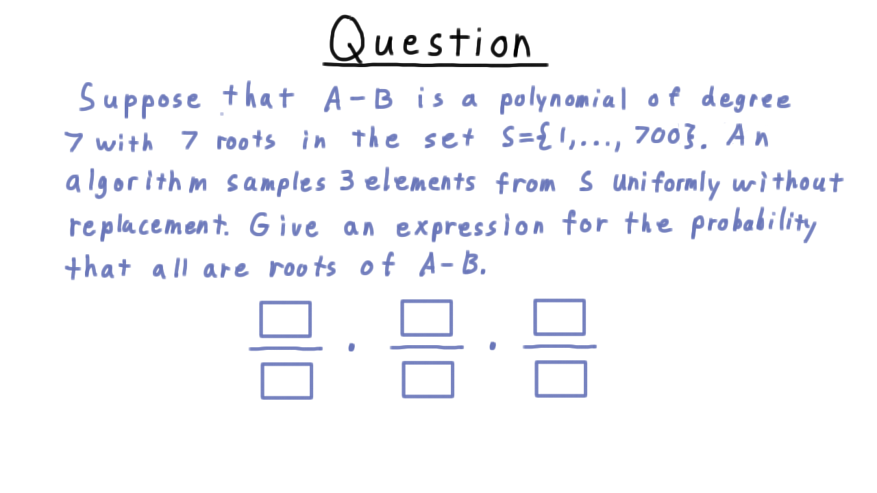
Quiz: Compute the success probability when sampling without replacement.
Random Variables and Expectation
A random variable \(X : \Omega \to \mathbb{R}\) assigns a real value to each outcome.
Expectation:
Linearity of expectation (holds even for dependent random variables):
This is the key tool for analyzing randomized algorithms.
Randomized Quicksort
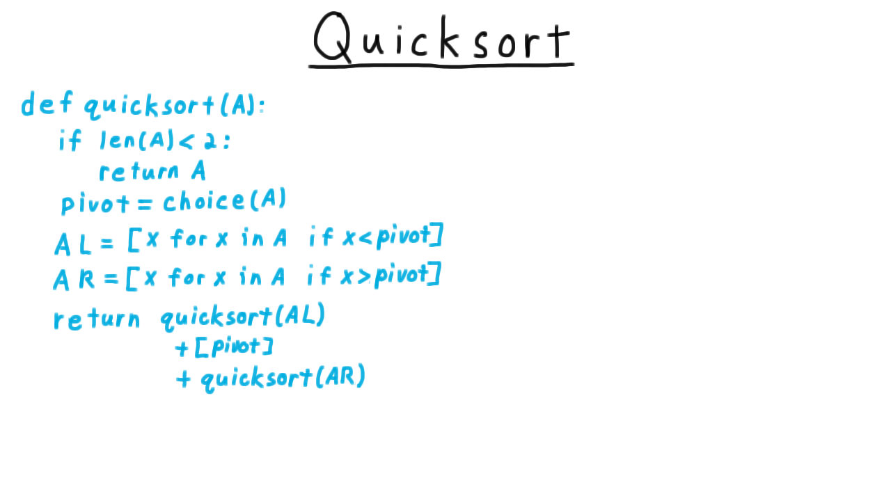
Quicksort pseudocode with random pivot selection.
Best case (ideal pivots): \(O(n \log n)\)
Worst case (always min/max pivot): \(O(n^2)\)
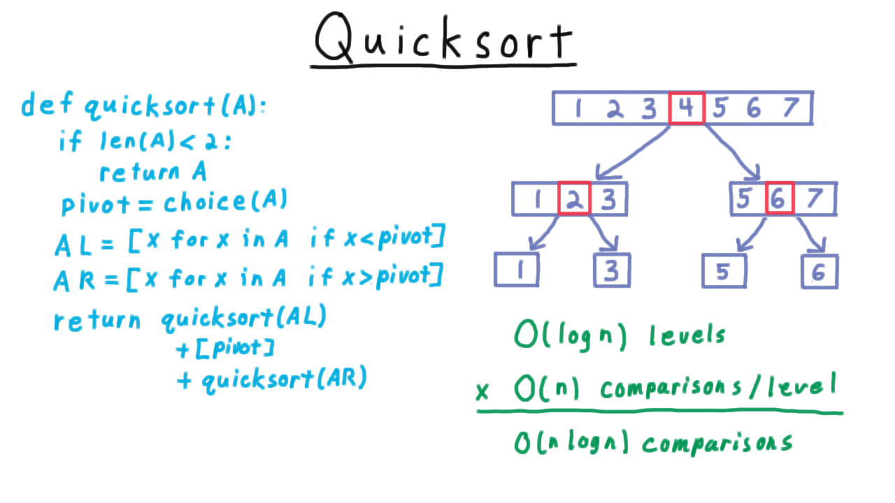
Balanced recursion tree with near-median pivots.
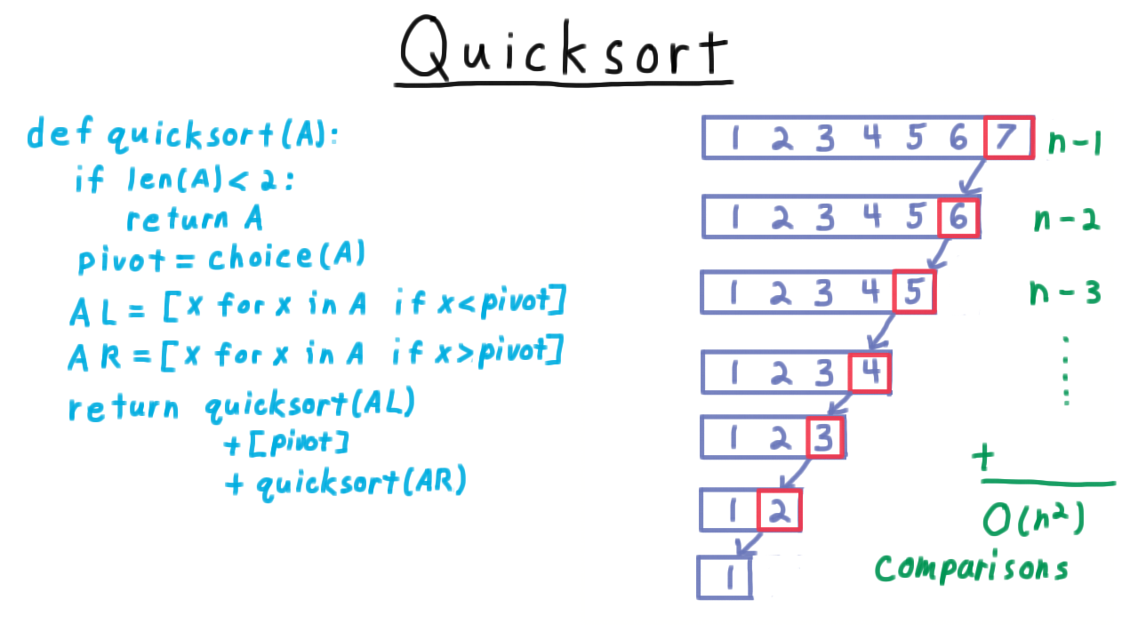
Unbalanced recursion tree when the pivot is always extreme.
Expected-Case Analysis
Let \(X_{ij} = 1\) if elements \(z_i\) and \(z_j\) (with \(i < j\)) are ever compared, and 0 otherwise.
Two elements \(z_i\) and \(z_j\) are compared if and only if one of them is chosen as the pivot before any element strictly between them. By symmetry:
Total expected comparisons:
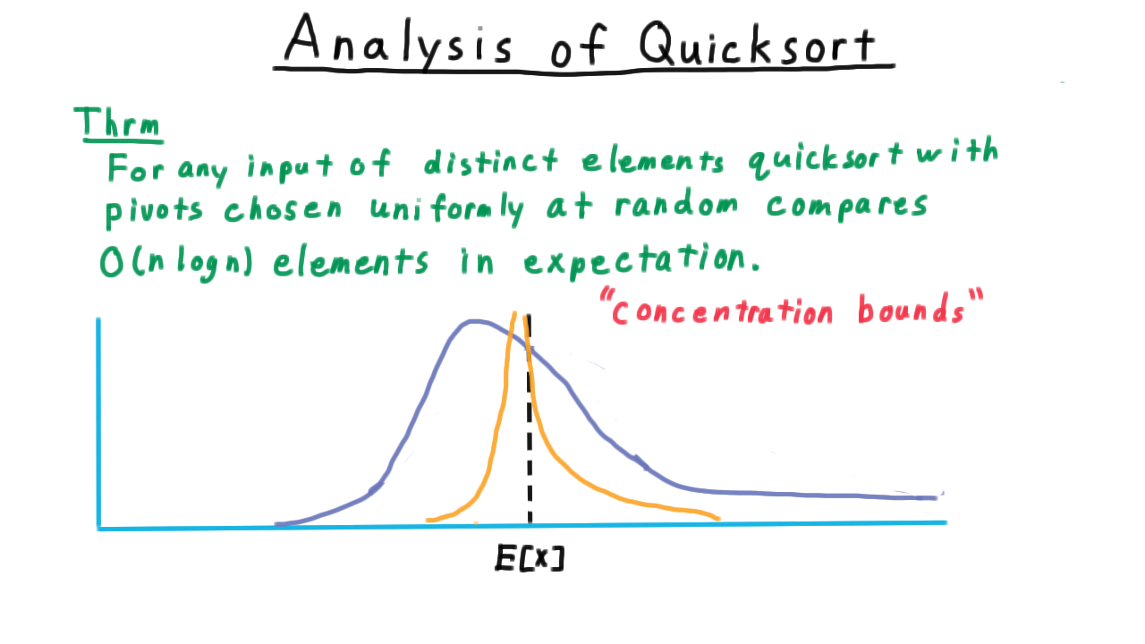
Running time concentrates tightly around \(O(n \log n)\) — large deviations are exponentially unlikely.
Karger’s Minimum Cut Algorithm
Problem: Given an undirected graph \(G = (V, E)\), find the minimum-sized set of edges whose removal disconnects \(G\).
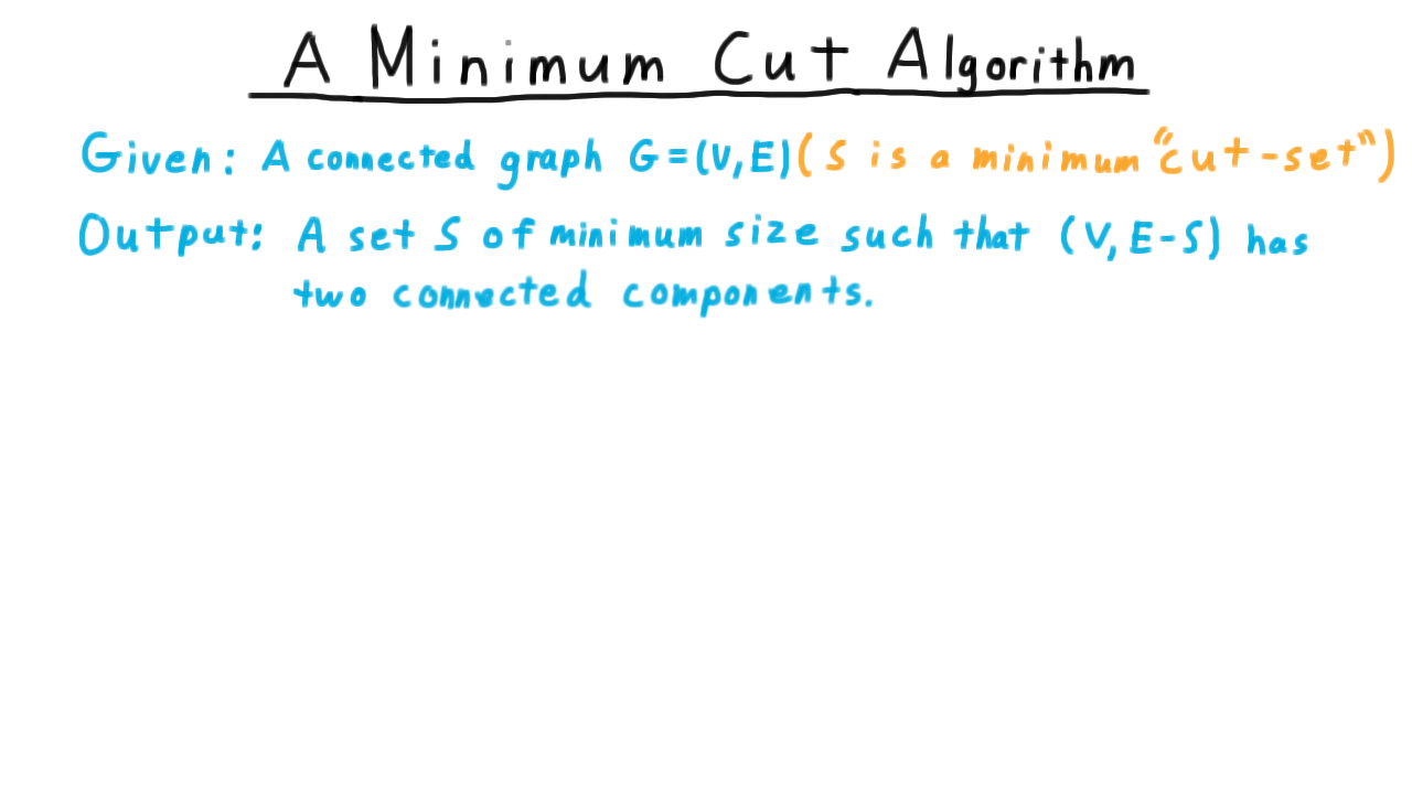
Definition of a minimum cut.
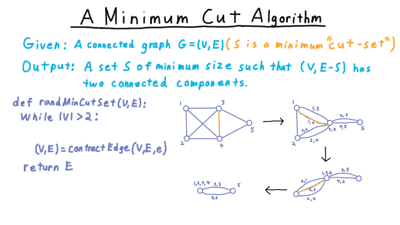
Edge contraction example — merging two vertices into one.
Algorithm (Karger’s contraction):
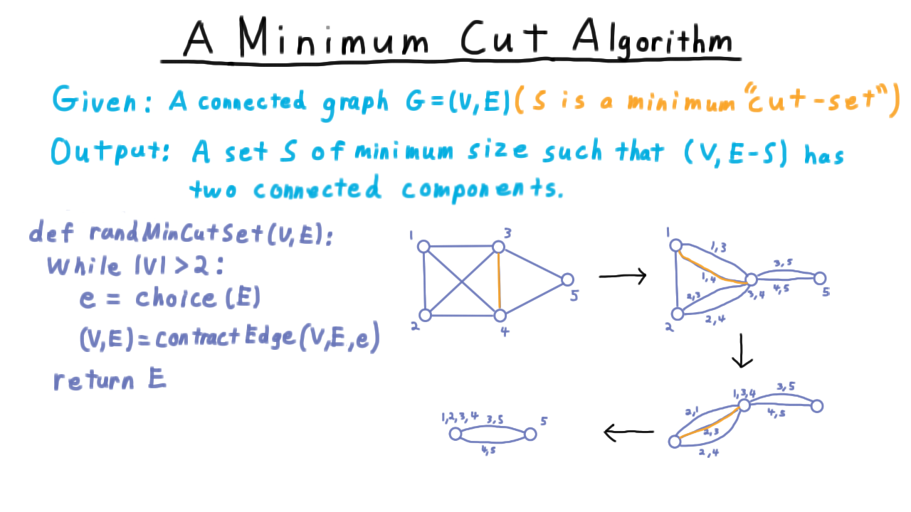
Karger’s algorithm pseudocode.
while |V| > 2:
    pick a random edge (u, v)
    contract u and v into a single vertex
    remove self-loops
return the remaining edges (the cut)
Success Probability
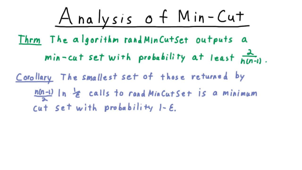
Probability analysis for Karger’s algorithm.
Let \(C\) be a minimum cut of size \(k\). At contraction step \(j\) (when \(n - j\) vertices remain), the probability that no edge of \(C\) is contracted is:
Telescoping over all \(n - 2\) steps:
Amplification: Run \(n(n-1)\ln(1/\varepsilon)\) independent trials and return the smallest cut found. Failure probability drops to at most \(\varepsilon\):
Maximum 3-SAT
Problem: Given a 3-CNF formula with \(m\) clauses, find an assignment maximising the number of satisfied clauses.
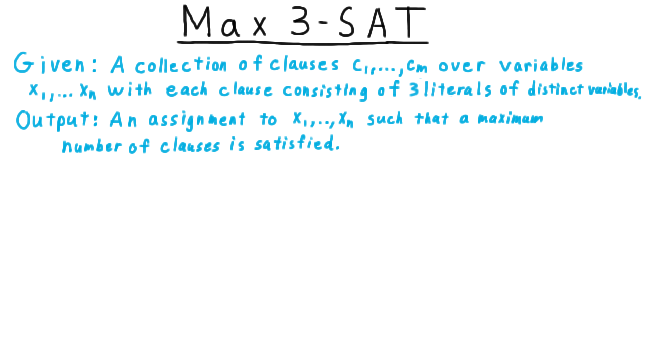
Maximum 3-SAT problem definition.
Theorem: Every 3-CNF formula has an assignment satisfying at least \(7m/8\) clauses.
Proof via expectation: Each clause has exactly one out of \(2^3 = 8\) assignments that fails it. For a uniformly random assignment:
By linearity of expectation:
Since the expectation is \(7m/8\), some assignment must achieve at least this.
Expected number of satisfied clauses equals \(7m/8\).
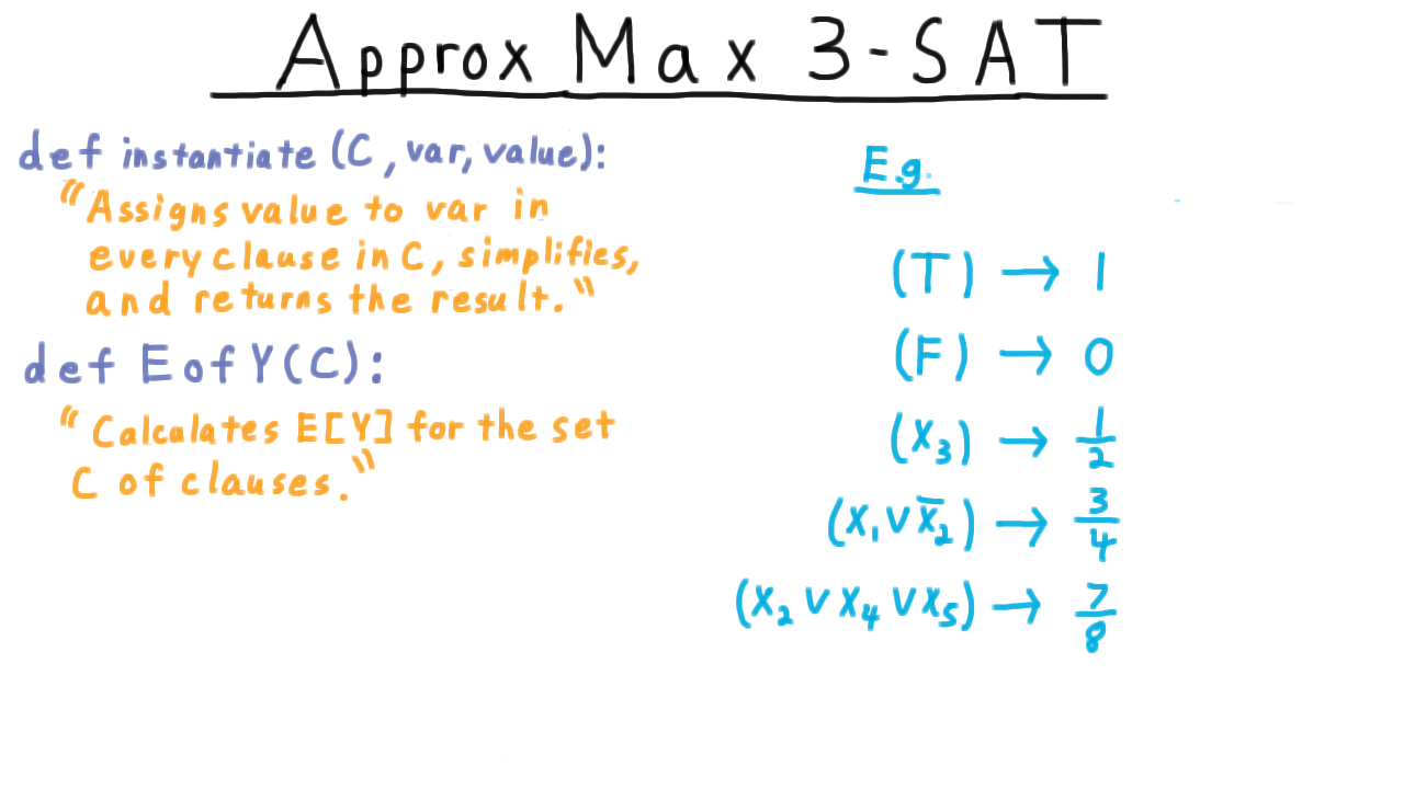
Derandomization via Method of Conditional Expectations
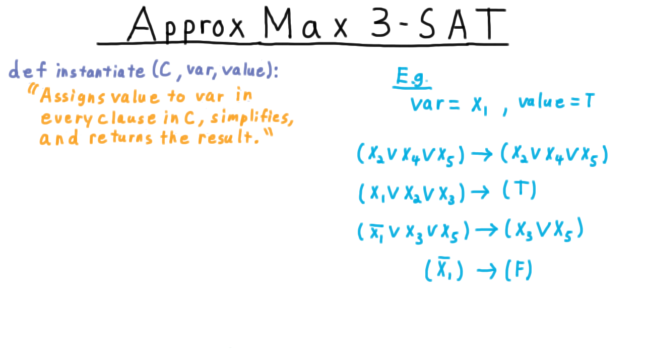
Instantiate one variable at a time, choosing the value that maximises the conditional expected number of satisfied clauses.
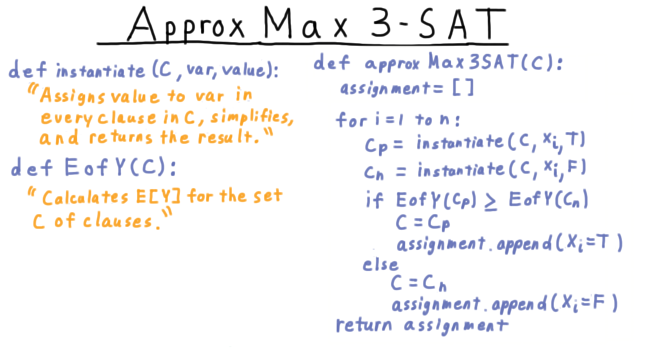
Derandomized Max-3-SAT algorithm pseudocode.
for each variable x_i:
    compute E[satisfied | x_1,...,x_{i-1}, x_i = True]
    compute E[satisfied | x_1,...,x_{i-1}, x_i = False]
    set x_i to whichever gives the higher expectation
Invariant: At each step the conditional expectation \(\geq 7m/8\).
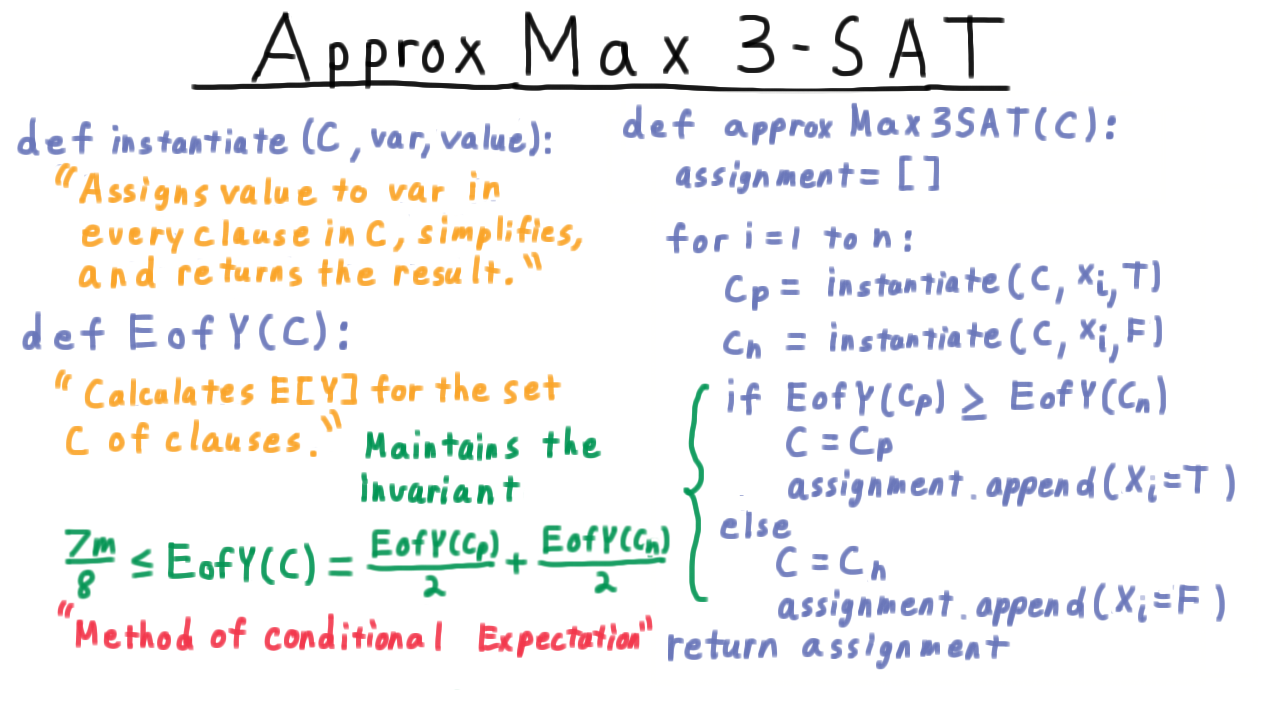
Analysis: the greedy choice maintains \(\geq 7m/8\) satisfied clauses throughout, giving a deterministic polynomial-time \(7/8\)-approximation.
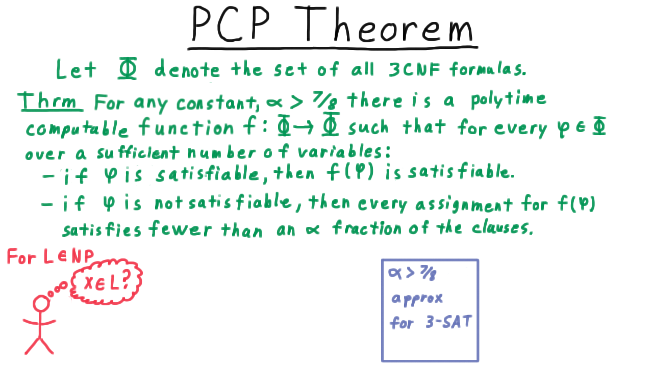
Hardness of Approximation and the PCP Theorem
Question: Can we do better than \(7/8\) for Max-3-SAT?
Setup: what does a better approximation imply?
PCP Theorem: For any \(\alpha > 7/8\) there exists a polynomial-time reduction \(f\) mapping 3-CNF formulas such that:
Satisfiable formulas map to satisfiable formulas.
Unsatisfiable formulas map to instances where no assignment satisfies more than an \(\alpha\) fraction of clauses.
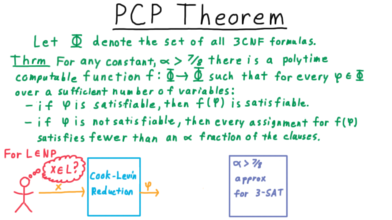
Apply Cook-Levin to reduce an arbitrary NP language to SAT.
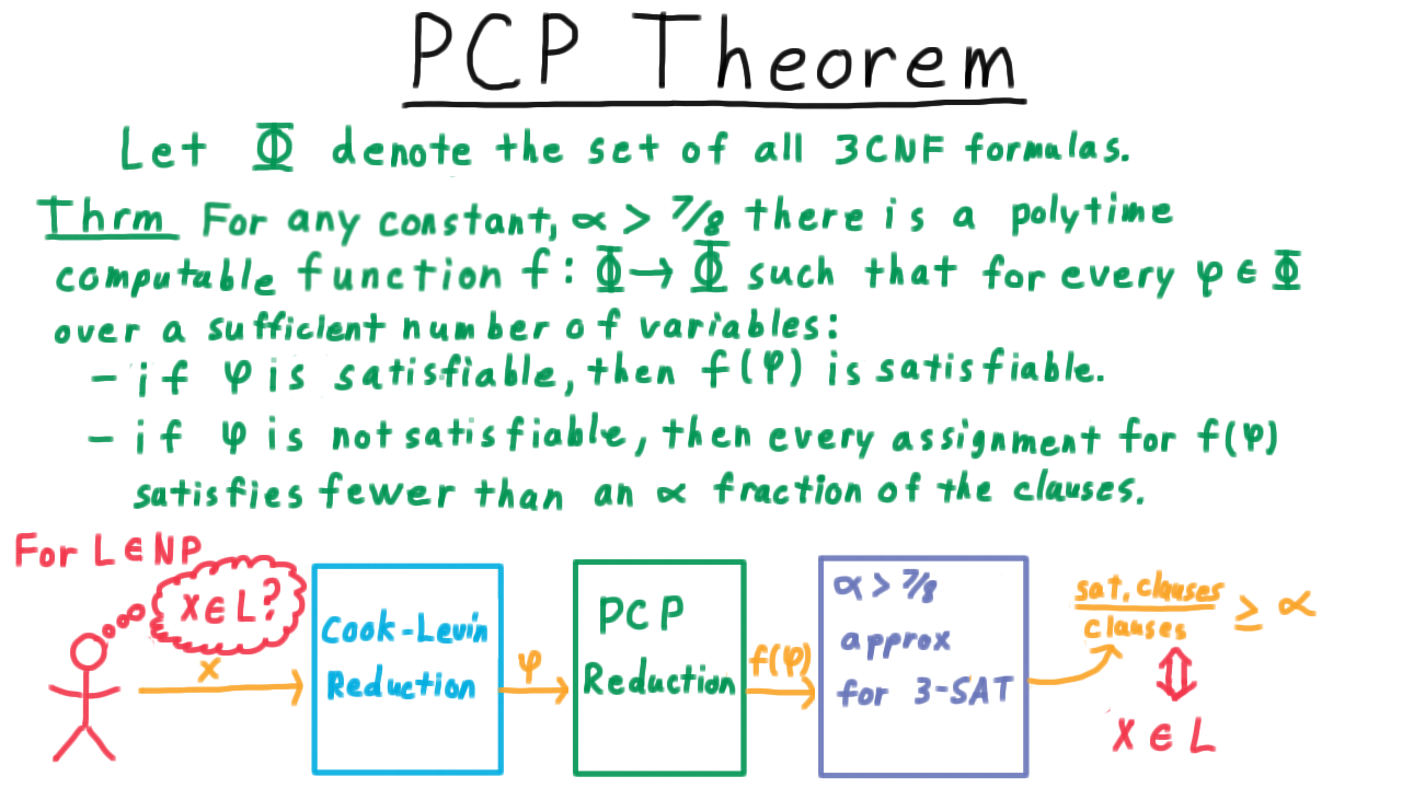
Apply the PCP transformation, then use the approximation algorithm to distinguish the two cases — solving NP-complete problems in polynomial time.
Conclusion: An \(\alpha\)-approximation for Max-3-SAT with \(\alpha > 7/8\) would imply \(P = NP\). The \(7/8\) ratio is tight.
Complexity Classes
RP (Randomized Polynomial time): One-sided Monte Carlo algorithms; always correct on “No” instances, correct on “Yes” instances with probability \(\geq 1/2\).
BPP (Bounded-error Probabilistic Polynomial time): Two-sided Monte Carlo; correct on any instance with probability \(\geq 2/3\).
ZPP (Zero-error Probabilistic Polynomial time): Las Vegas algorithms with expected polynomial runtime.
Open question (P vs. BPP): Whether every language decidable by a two-sided Monte Carlo polynomial algorithm can also be decided deterministically in polynomial time remains unresolved.
Key Formulas
Polynomial identity testing error bound:
Linearity of expectation:
Quicksort expected comparisons:
Karger’s success probability:
Max-3-SAT expectation:
Further Reading
Chernoff bounds and tail inequalities for concentration results
Universal hashing and randomized data structures
Randomized rounding of LP relaxations
Lovász Local Lemma for sparse dependency graphs