Approximation Algorithms

From Computability, Complexity & Algorithms — Charles Brubaker and Lance Fortnow

Introduction

Approximation algorithms provide efficient solutions to NP-complete problems when polynomial-time exact solutions are unavailable. Rather than seeking an optimal answer, they guarantee a solution within a specific factor of optimality.

Core idea: We might not be able to find the minimum vertex cover in polynomial time, but we can find one that is at most twice as large as the optimal — in polynomial time.

When exact solutions appear intractable, ask: is an approximate solution good enough?

---

Minimum Vertex Cover Approximation

A vertex cover is a set \(C \subseteq V\) such that every edge has at least one endpoint in \(C\). The goal is to find the smallest such set.

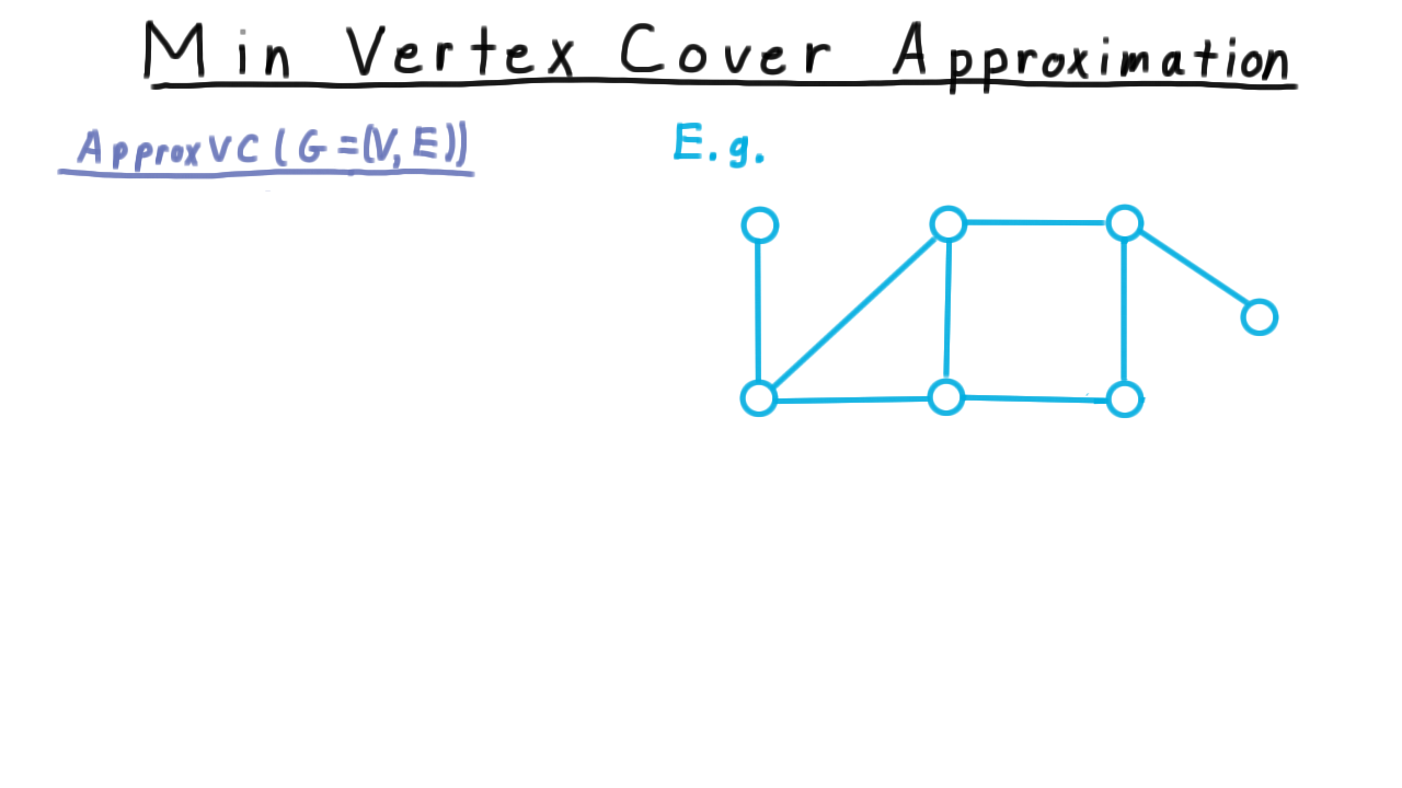
Definition of the minimum vertex cover problem.

ApproxVC Algorithm

C ← ∅
while uncovered edges exist:
    pick an arbitrary uncovered edge (u, v)
    add u and v to C
    remove all edges incident to u or v
return C

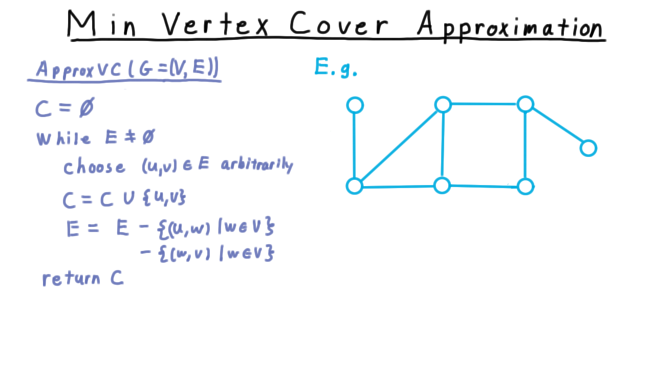
Steps of the ApproxVC algorithm.

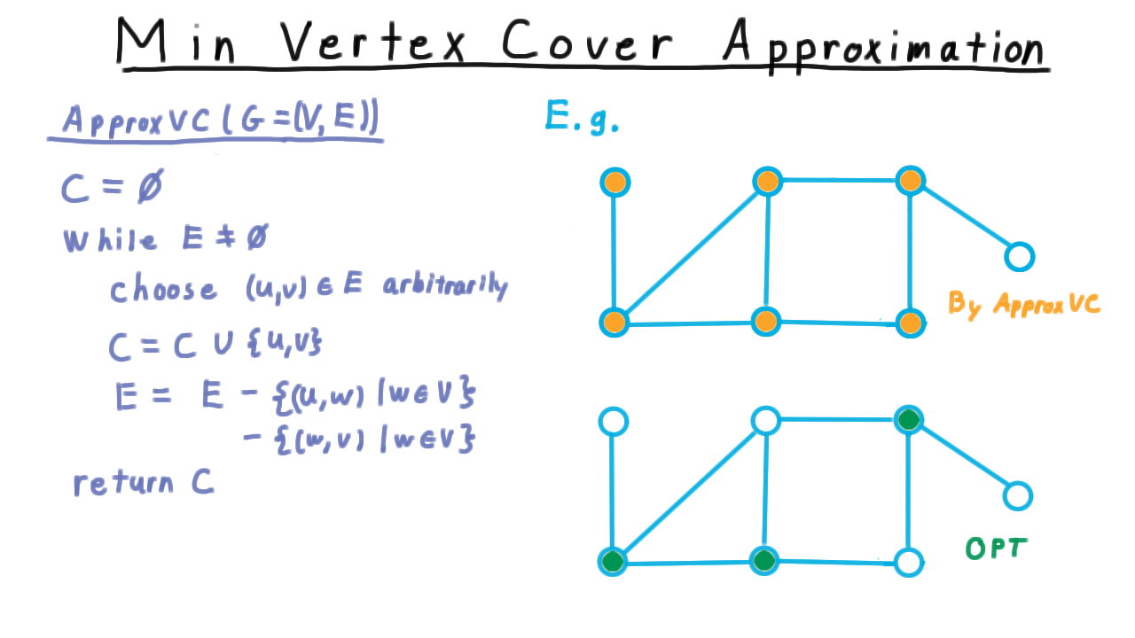
Algorithm output (orange) vs. optimal cover (green) — the approximation can be suboptimal but is always within a factor of 2.

Performance Guarantee

Theorem: ApproxVC returns \(C\) such that:

\[\frac{|C|}{|C^*|} \leq 2\]

where \(C^*\) is the minimum vertex cover.

Proof:

Let \(M\) be the set of edges selected by the algorithm (each chosen edge is added to \(M\) before its endpoints are added to \(C\)). The edges in \(M\) form a maximal matching — no two share an endpoint.

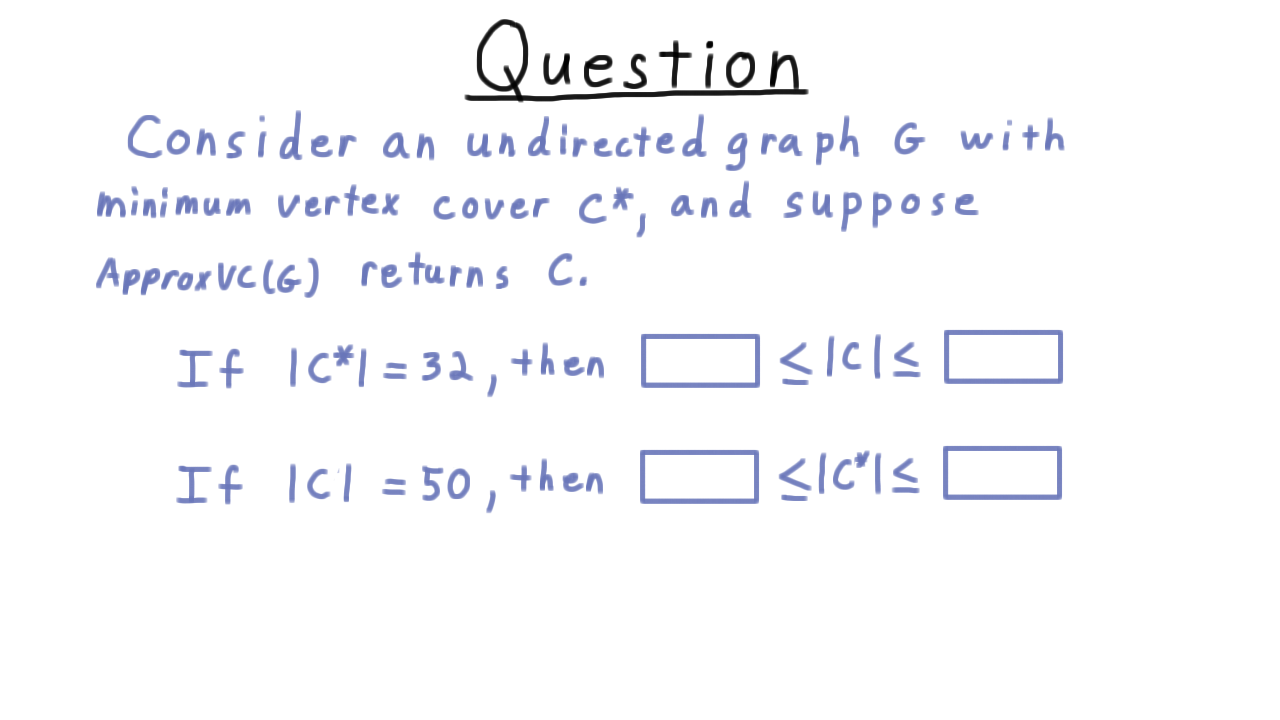
Quiz: Explore the relationship between \(C\) and \(C^*\).

The challenge is bounding \(|C^*|\) without knowing it directly.

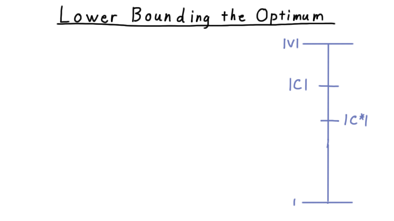
How do we bound the optimum when we don’t know it?

Use a lower bound on \(|C^*|\) to bound the ratio.

Key observations:

1. Any vertex cover must include at least one endpoint from each edge in \(M\), and since no two edges in \(M\) share a vertex:

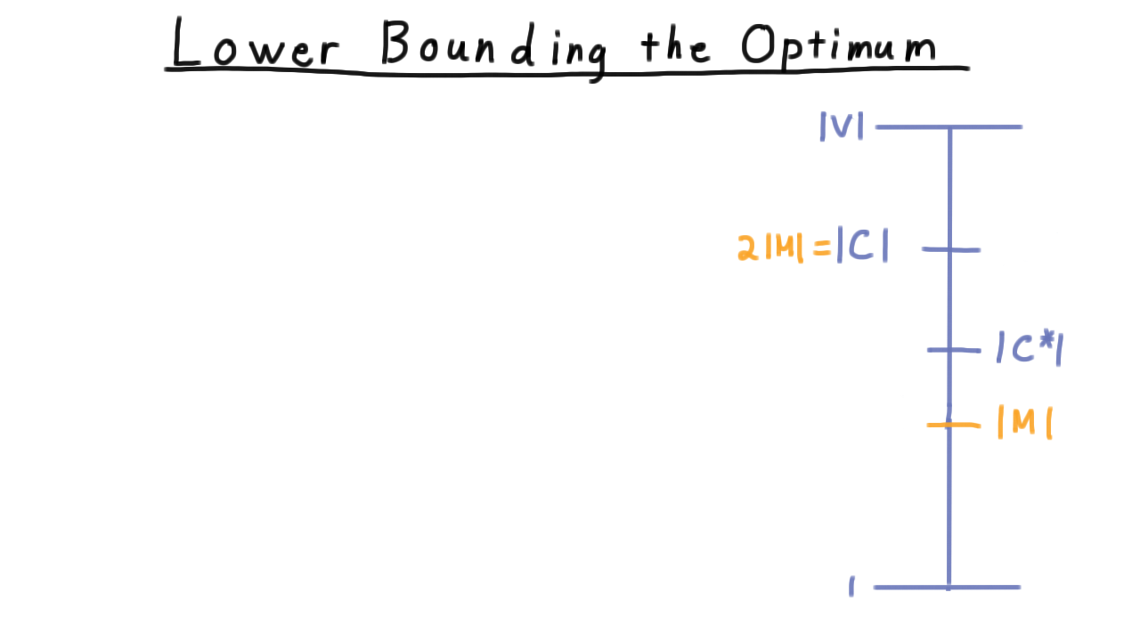
   \[|M| \leq |C^*|\]

2. The algorithm adds exactly 2 vertices per selected edge:

   \[|C| = 2|M|\]

3. Combining:

   \[|C| = 2|M| \leq 2|C^*|\]

Tightness

The factor-2 bound is tight — there exist graphs where the algorithm returns a cover exactly twice the size of the optimal.

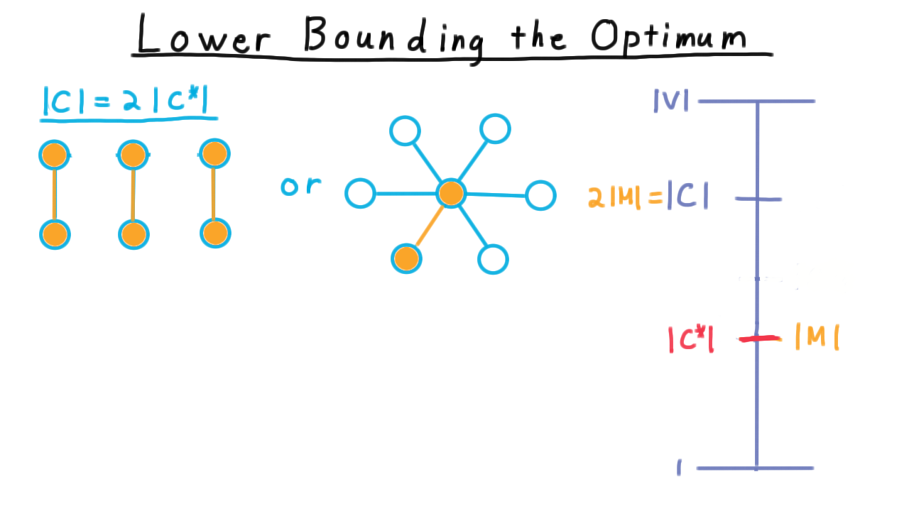
Scenario where the approximation is exactly twice the optimal.

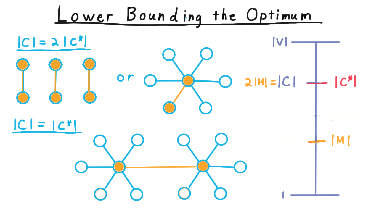
Scenario where the algorithm finds an exact optimal solution.

---

Formal Definitions

Optimization Problems

An optimization problem consists of:

1. A set of valid instances (inputs).

2. A set of feasible solutions for each instance.

3. An objective function to minimize or maximize.

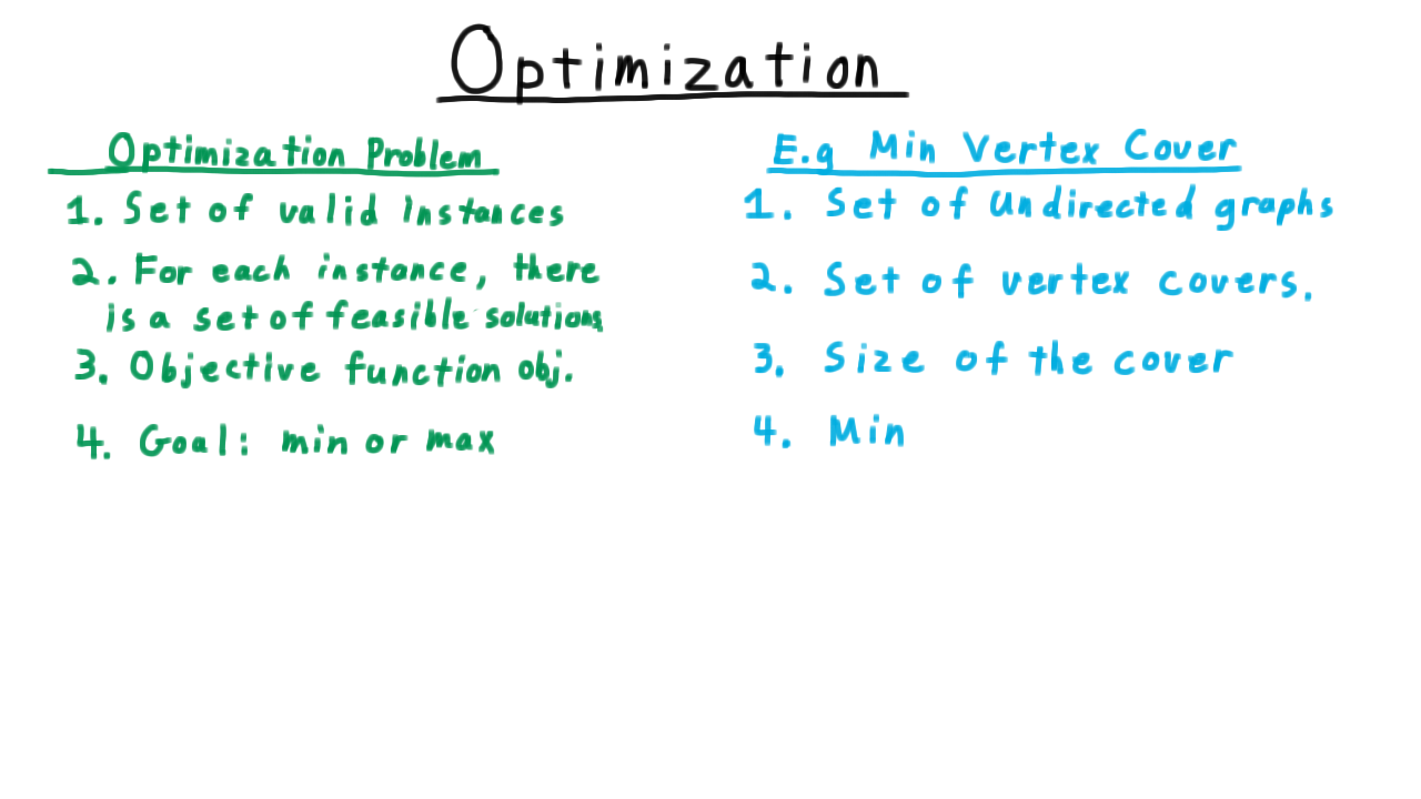
Formal definition of an optimization problem.

An NP-optimization problem is one where all three components are computable in polynomial time.

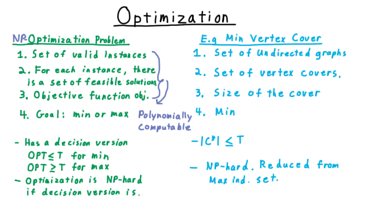
NP-optimization: instances, solutions, and objective all poly-time computable.

Approximation Algorithm Definition

Algorithm \(A\) is a factor-\(\delta\) approximation for a minimization problem if it runs in polynomial time and for every instance \(I\):

\[\frac{|A(I)|}{|OPT(I)|} \leq \delta\]

For a maximization problem the inequality reverses:

\[\frac{|A(I)|}{|OPT(I)|} \geq \delta\]

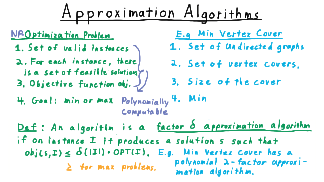
Formal definition of a factor-\(\delta\) approximation algorithm.

---

Subset Sum: An FPTAS

Problem: Given a set of integers and a threshold \(t\), find a subset maximizing the sum without exceeding \(t\).

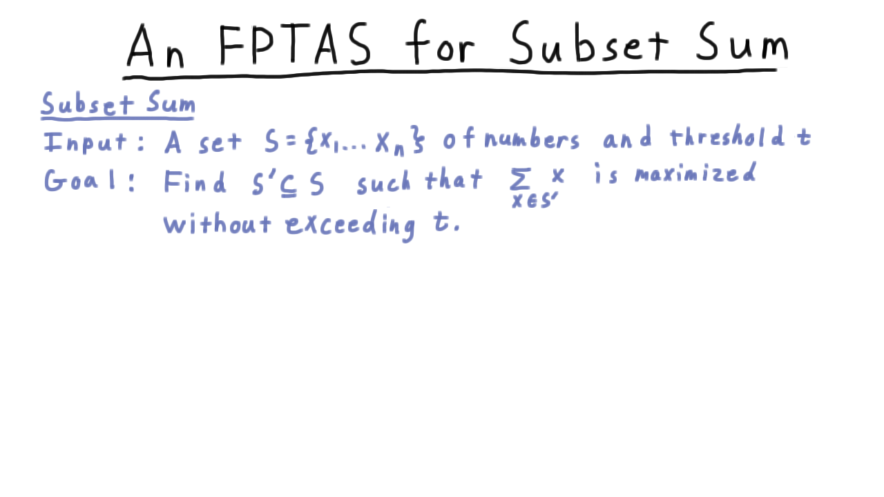
Formal definition of the subset sum optimization problem.

Key result: For any \(\varepsilon > 0\) there is an algorithm running in \(O\!\left(\frac{n^2 \log t}{\varepsilon}\right)\) time that is a factor \((1+\varepsilon)^{-1}\) approximation.

Classification:

• PTAS (Polynomial Time Approximation Scheme): Running time polynomial in \(n\) for every fixed \(\varepsilon > 0\).

• FPTAS (Fully Polynomial Time Approximation Scheme): Running time polynomial in both \(n\) and \(1/\varepsilon\).

FPTAS is the strongest class of approximation result — subset sum admits one.

---

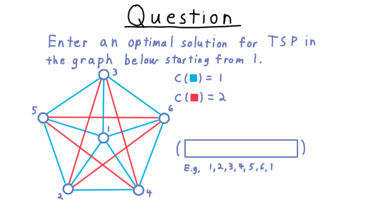
Traveling Salesman Problem

Problem: Given a complete weighted graph, find the minimum-cost Hamiltonian cycle (a cycle visiting every vertex exactly once).

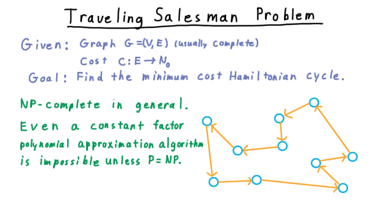
Formal definition of the Traveling Salesman Problem.

Hardness of Approximation (General TSP)

Theorem: Unless \(P = NP\), no constant-factor polynomial-time approximation exists for general TSP.

Proof (reduction from Hamiltonian Cycle):

Given graph \(G = (V, E)\), construct a complete weighted graph \(G'\):

\[\begin{split}w(u,v) = \begin{cases} 1 & \text{if } (u,v) \in E \\ \alpha|V| + 1 & \text{if } (u,v) \notin E \end{cases}\end{split}\]

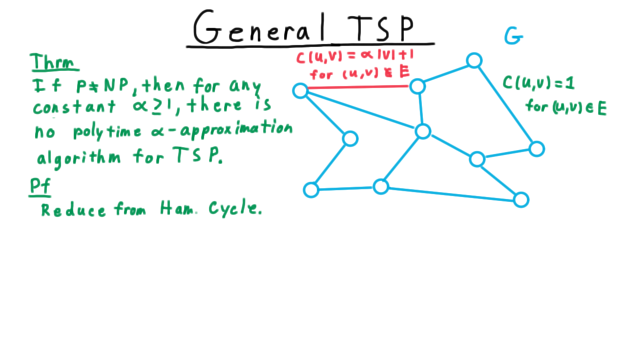
Reduction from Hamiltonian Cycle to TSP by assigning edge weights.

Analysis:

• If \(G\) has a Hamiltonian cycle: optimal TSP cost \(= |V|\).

• If \(G\) has no Hamiltonian cycle: every tour uses at least one non-\(E\) edge, so cost \(\geq (1 + \alpha)|V|\).

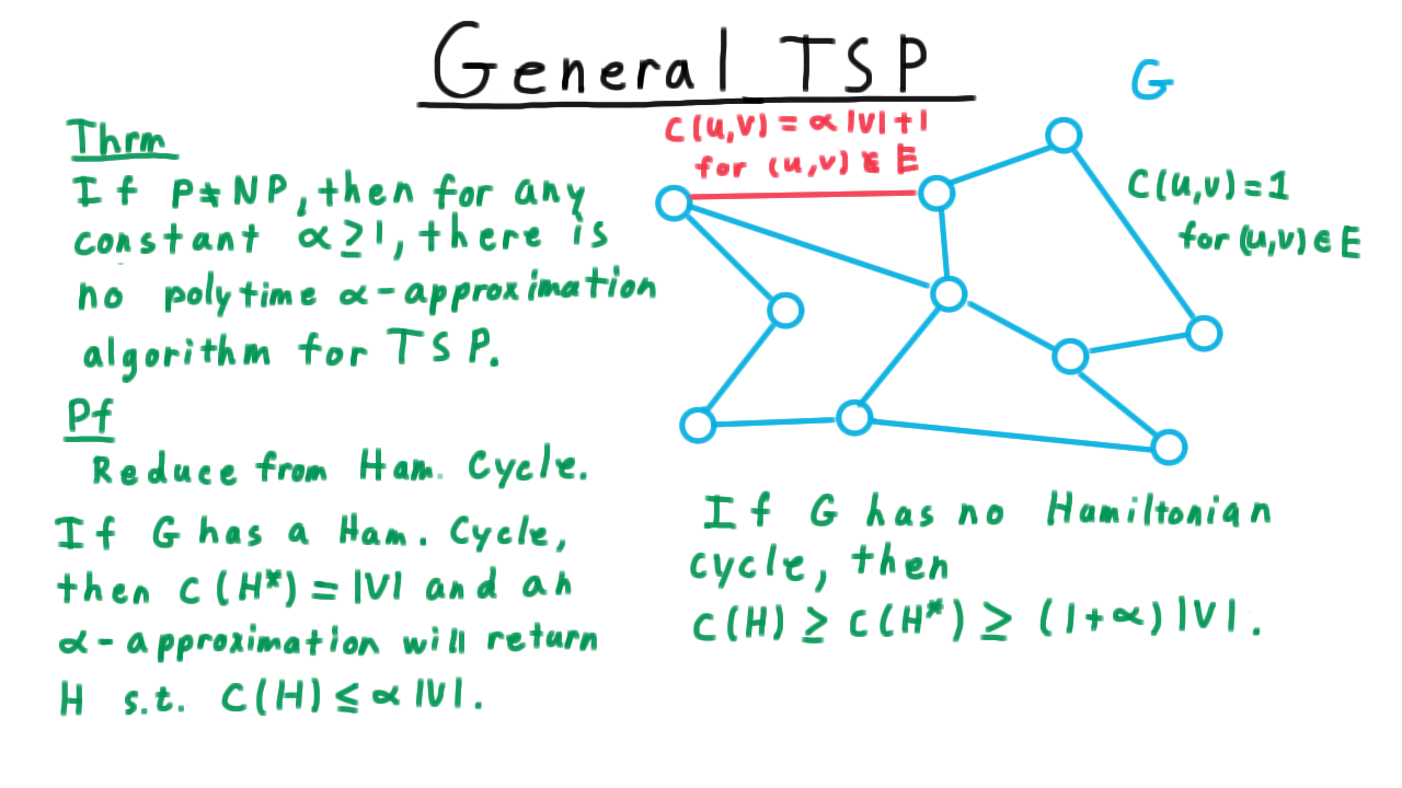
A factor-\(\alpha\) approximation would distinguish the two cases, solving an NP-complete problem in polynomial time.

A factor-\(\alpha\) approximation algorithm would separate these two cases, which would place Hamiltonian Cycle in P — contradicting \(P \neq NP\).

Conclusion: General TSP is inapproximable to any constant factor unless \(P = NP\).

---

Metric TSP

Restriction: Require the edge weights to satisfy the triangle inequality:

\[w(u, v) \leq w(u, x) + w(x, v) \quad \forall\, u, v, x \in V\]

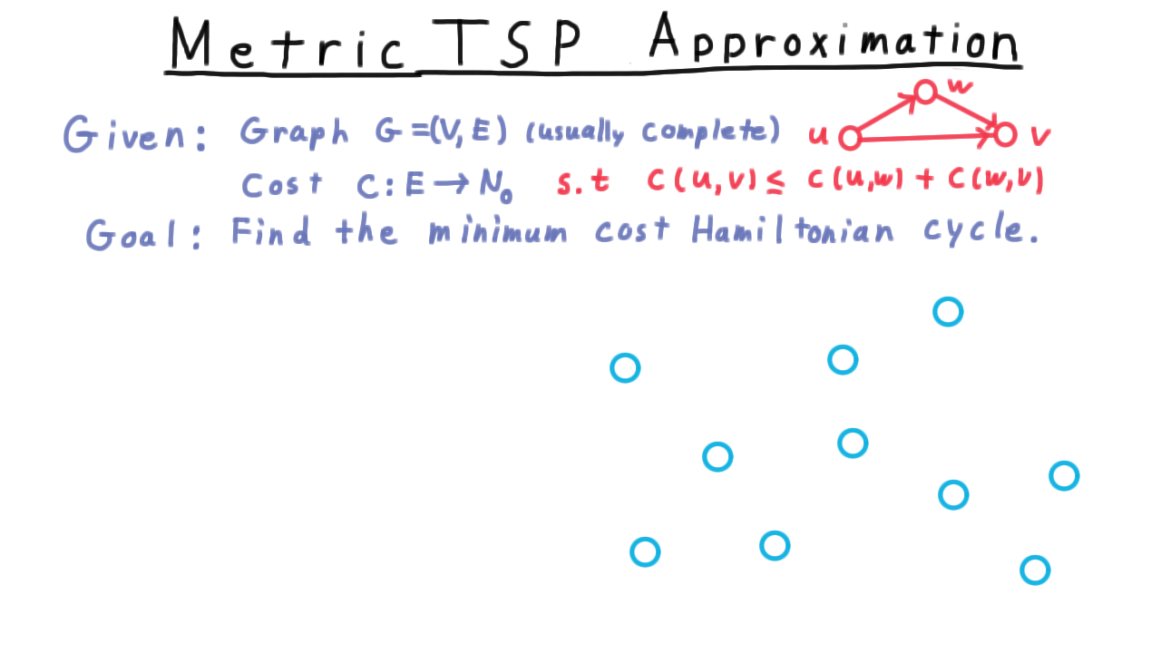
Definition of metric TSP with the triangle inequality constraint.

ApproxMetricTSP Algorithm

1. Build a minimum spanning tree T (Kruskal or Prim)
2. Perform a depth-first search on T
3. Output vertices in DFS discovery order as the tour

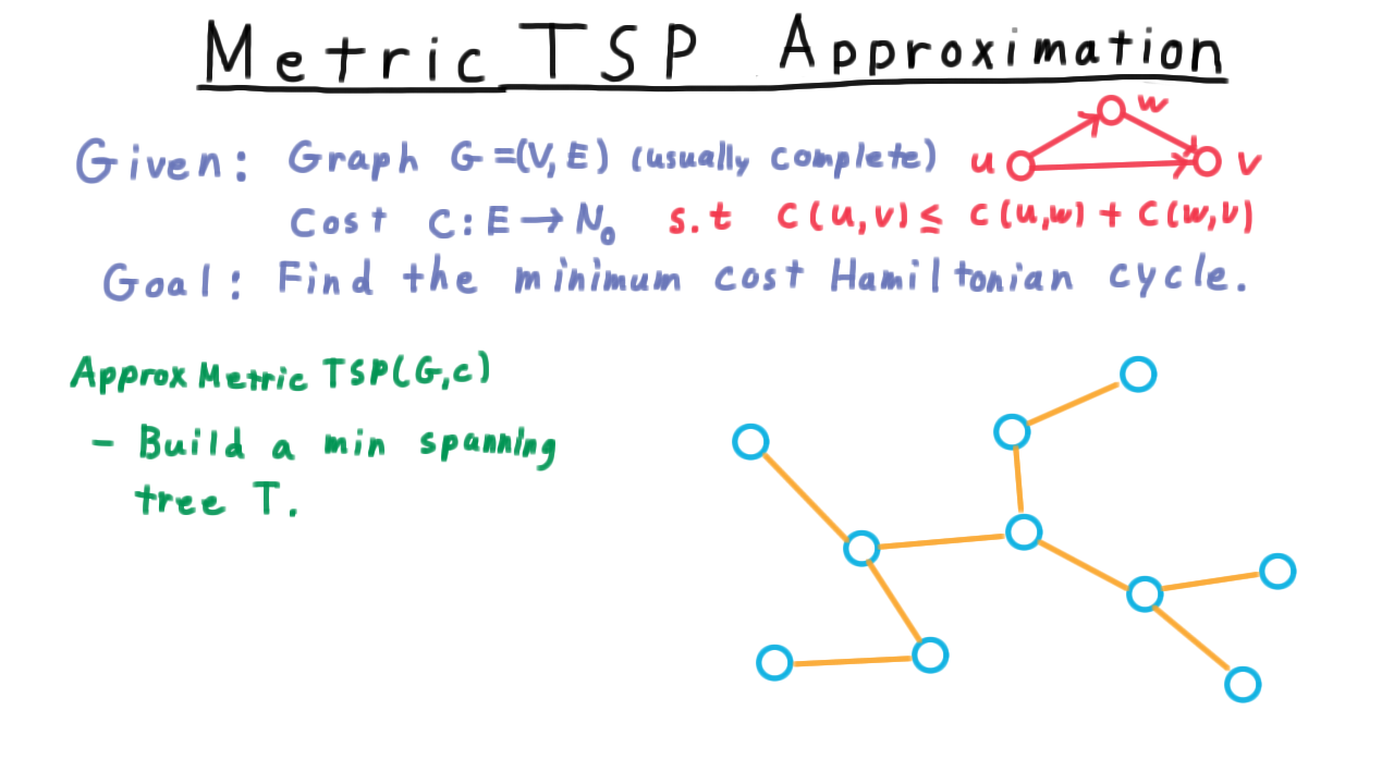
Step 1: Construct the minimum spanning tree \(T\).

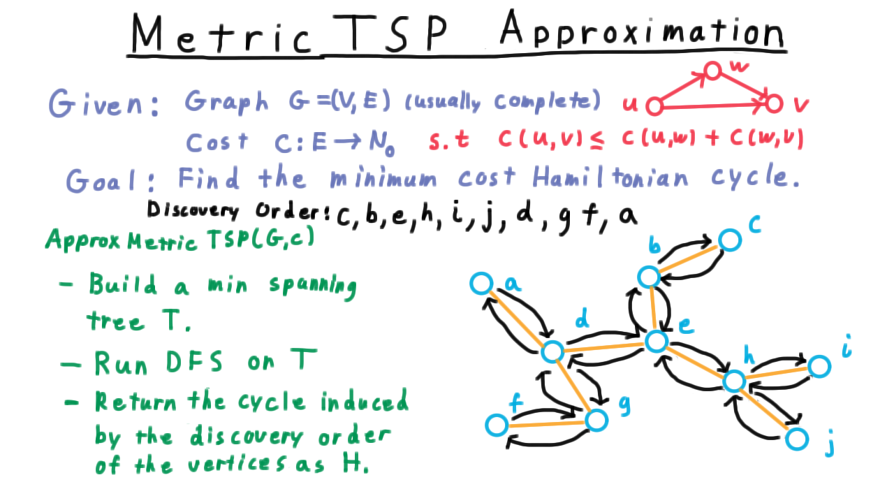
Step 2–3: DFS discovery order gives the approximate tour.

Running time: \(O(V^2)\) (dominated by MST construction on a complete graph).

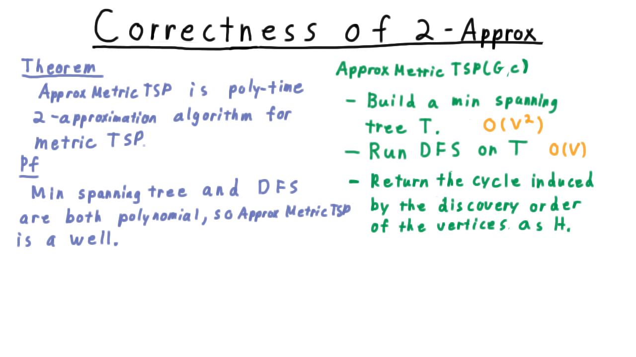
Time complexity analysis of ApproxMetricTSP.

Performance Guarantee

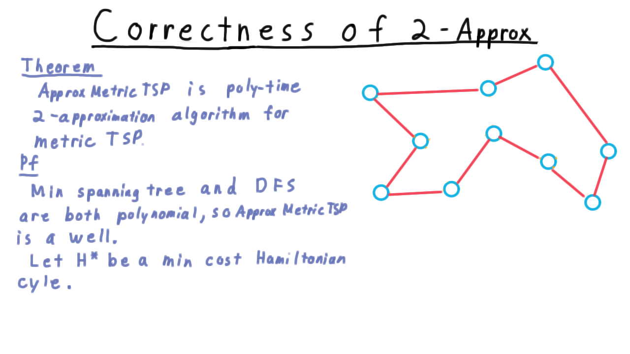
Theorem: ApproxMetricTSP is a factor-2 approximation for metric TSP.

Example graph used in the correctness proof.

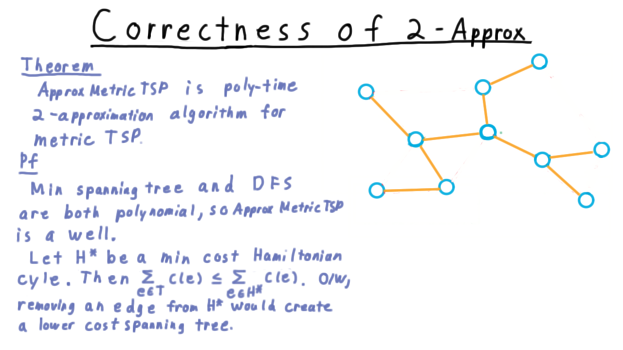
Minimum spanning tree constructed from the example graph.

Proof:

Let \(T\) be the MST and \(OPT\) be the optimal tour cost.

1. MST cost \(\leq OPT\): Removing any single edge from the optimal tour yields a spanning tree, so \(w(T) \leq OPT\).

2. DFS traversal cost \(= 2 \cdot w(T)\): A full DFS traversal visits every edge of \(T\) exactly twice.

3. Shortcutting repeated vertices (skipping already-visited nodes) does not increase cost under the triangle inequality.

Therefore:

\[w(\text{tour}) \leq 2 \cdot w(T) \leq 2 \cdot OPT\]

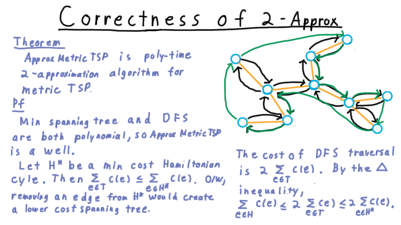
Visualization of the factor-2 approximation proof.

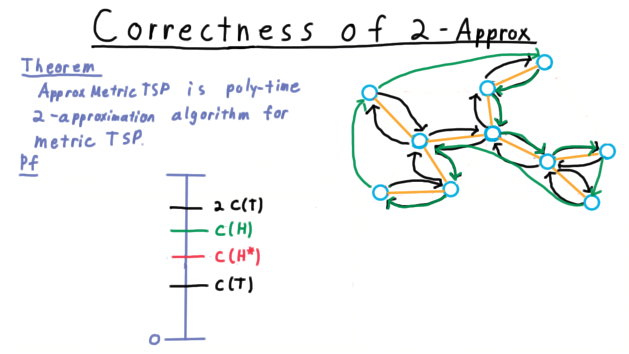
Scale illustration of the cost relationships: \(w(\text{tour}) \leq 2 \cdot w(T) \leq 2 \cdot OPT\).

Tightness of the Factor-2 Bound

Quiz: Analyze the tightness of the approximation on this example.

Consider a star graph with one center and \(n-1\) leaves, where edge weights satisfy the triangle inequality:

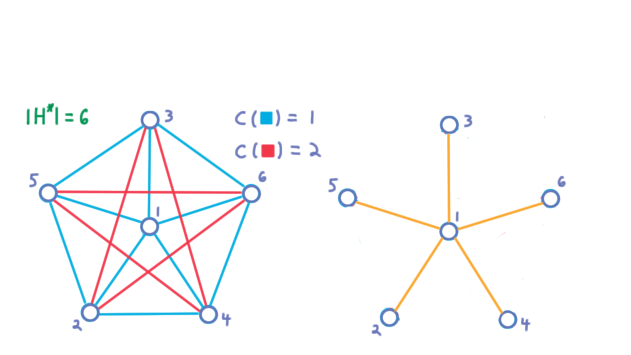
Star-shaped MST: center connected to all \(n-1\) leaves.

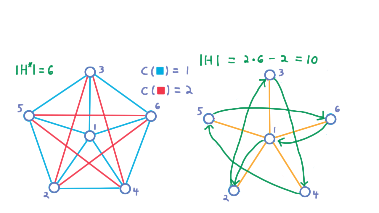
Resulting DFS tour — the algorithm’s cost approaches \(2 \cdot OPT\) as \(n \to \infty\).

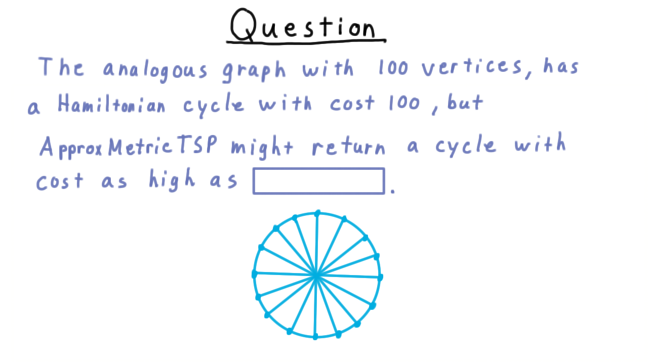
Quiz: What is the worst-case approximation ratio for 100 vertices on this graph?

The bound is tight: for any \(n\), there exist metric instances where ApproxMetricTSP returns a tour of cost approaching \(2 \cdot OPT\).

---

Summary of Results

Problem	Result	Notes
Min Vertex Cover	Factor-2 approximation	Tight; uses maximal matching lower bound
Subset Sum	FPTAS \((1+\varepsilon)^{-1}\)	Poly in \(n\) and \(1/\varepsilon\)
General TSP	Inapproximable (any constant)	Unless \(P = NP\)
Metric TSP	Factor-2 approximation	Tight; uses MST lower bound

---

Key Formulas

\[\frac{|A(I)|}{|OPT(I)|} \leq \delta \quad \text{(factor-}\delta\text{ approximation, minimization)}\]

\[|C| = 2|M| \leq 2|C^*| \quad \text{(vertex cover approximation ratio)}\]

\[w(T) \leq OPT \leq w(\text{tour}) \leq 2 \cdot w(T) \quad \text{(metric TSP proof chain)}\]

\[w(u,v) \leq w(u,x) + w(x,v) \quad \text{(triangle inequality)}\]

---

Further Reading

• Christofides algorithm: factor-\(\frac{3}{2}\) approximation for metric TSP

• MAX-3SAT: randomized constant-factor approximation

• Hardness of approximation via PCP theorem