Dynamic Programming

From Computability, Complexity & Algorithms — Charles Brubaker and Lance Fortnow

Introduction

Dynamic programming is a design technique for solving optimization problems efficiently by exploiting optimal substructure — expressing a hard problem as combinations of optimal solutions to smaller, similar subproblems.

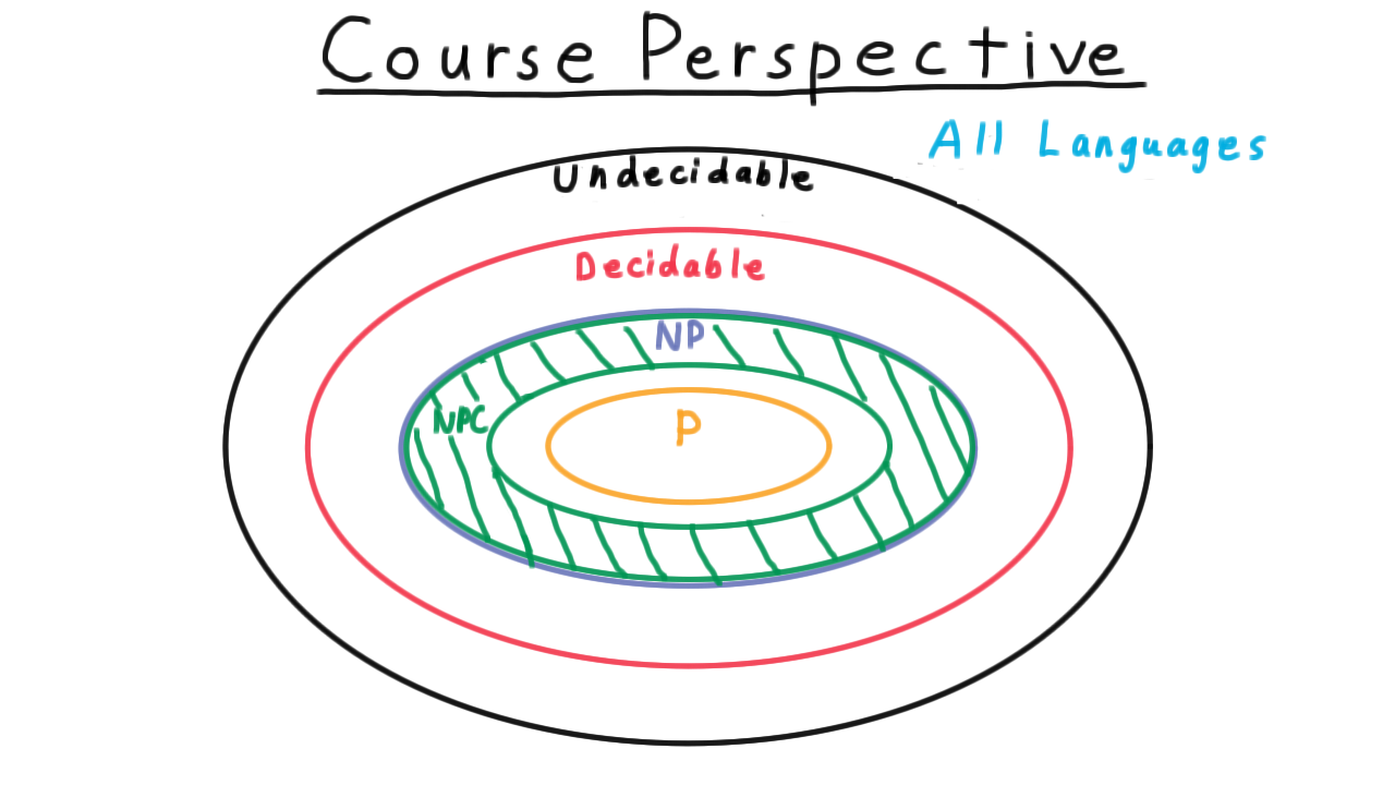
Context: polynomial-time algorithms sit inside the broader landscape of decidable, NP, and NP-complete problems.

Rather than recomputing subproblems via naive recursion, DP either:

• Memoizes results on first computation, or

• Fills a table in dependency order (bottom-up).

Motivating example — Fibonacci: Computing \(F(n) = F(n-1) + F(n-2)\) naively recomputes each subproblem roughly \(\varphi^k\) times (where \(\varphi\) is the golden ratio), giving exponential time. Filling a table bottom-up reduces this to \(O(n)\).

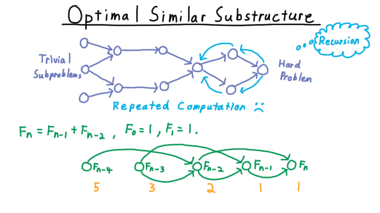
Recursion tree for Fibonacci — identical subtrees are recomputed repeatedly.

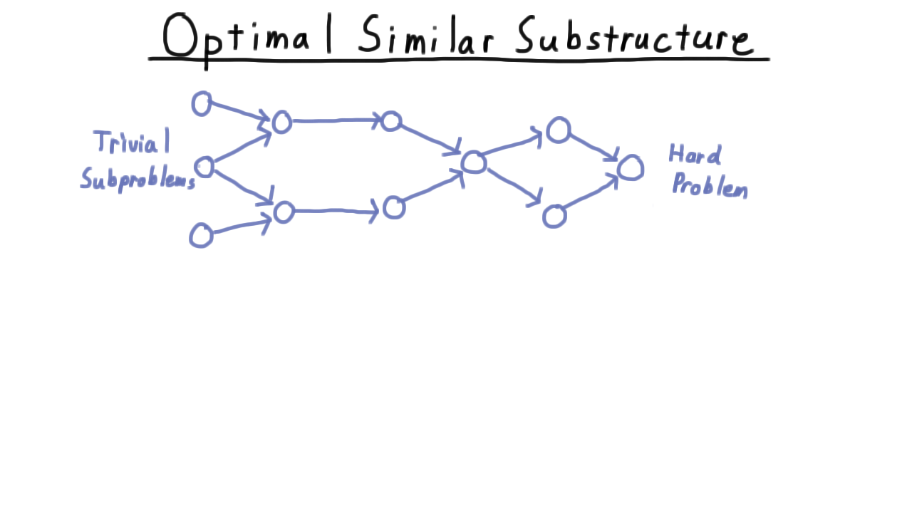
Subproblem dependency DAG — solving in topological order avoids redundant work.

---

Problem 1: Sequence Alignment (Edit Distance)

Goal: Find the minimum-cost alignment between two sequences \(X\) and \(Y\) (e.g., DNA strings).

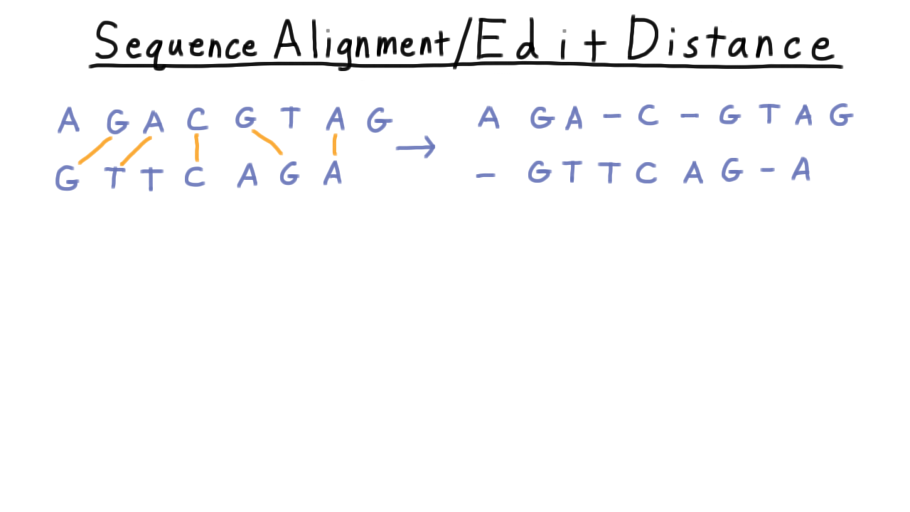
Example alignment between two genetic sequences.

Cost Function

An alignment \(A\) pairs characters from \(X\) and \(Y\) (possibly with gaps). The total cost combines:

• Gap penalty for unmatched characters (insertions / deletions): \(n + m - 2|A|\)

• Mismatch penalty for matched-but-different characters: \(\sum_{(i,j)\in A} \alpha(X_i, Y_j)\)

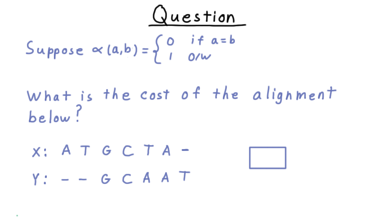
Quiz: Calculate the alignment cost for a given pair of sequences.

Recurrence

Let \(c(i, j)\) = minimum cost of aligning the first \(i\) characters of \(X\) with the first \(j\) characters of \(Y\).

At each step there are three cases:

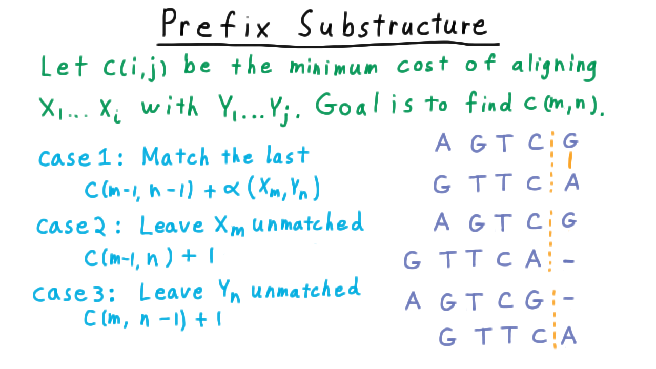
Three cases: match/mismatch the last characters, or introduce a gap in \(X\) or \(Y\).

\[\begin{split}c(i, j) = \min \begin{cases} c(i-1,\, j-1) + \alpha(X_i,\, Y_j) & \text{(match/mismatch last chars)} \\ c(i-1,\, j) + 1 & \text{(gap in } Y \text{)} \\ c(i,\, j-1) + 1 & \text{(gap in } X \text{)} \end{cases}\end{split}\]

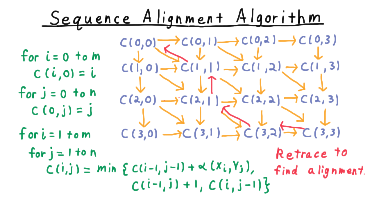
Base cases:

\[c(0, j) = j \qquad c(i, 0) = i\]

Algorithm

Fill an \((m+1) \times (n+1)\) grid in row-major (scanline) order so that \(c(i-1, j-1)\), \(c(i-1, j)\), and \(c(i, j-1)\) are always available.

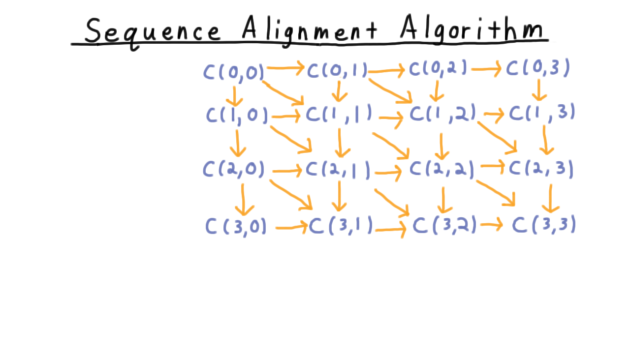
Grid structure — each cell depends on the cell above-left, above, and to the left.

Pseudocode for the sequence alignment / edit-distance algorithm.

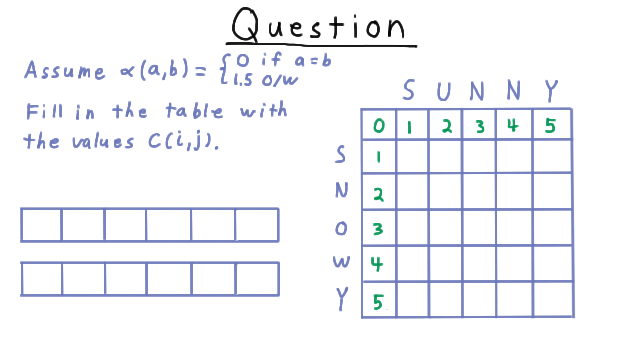
Quiz: Align "snowy" with "sunny" using the recurrence.

Backtrack through the table to reconstruct the actual alignment.

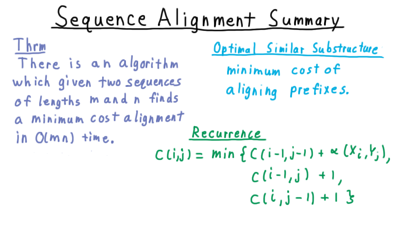
Summary: \(O(mn)\) time and space; backtracking gives the optimal alignment.

Time complexity: \(O(mn)\)

---

Problem 2: Chain Matrix Multiplication

Goal: Find the optimal parenthesization of a matrix chain \(A_1 \times A_2 \times \cdots \times A_n\) to minimize total scalar multiplications.

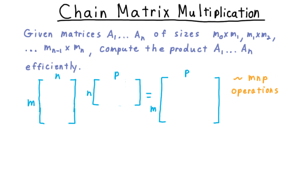
Multiplying an \(m \times n\) matrix by an \(n \times p\) matrix costs \(mnp\) scalar multiplications.

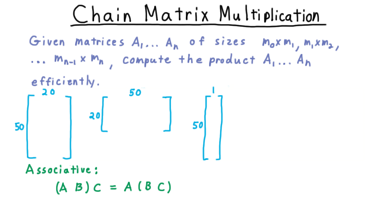
Two different parenthesizations of the same chain can differ dramatically in cost.

Key Insight

Matrix multiplication is associative but not commutative. The order of parenthesization does not change the result but can change the number of operations by orders of magnitude.

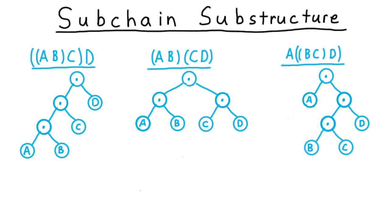
Expression trees for different parenthesizations of \(A_1 A_2 A_3 A_4\).

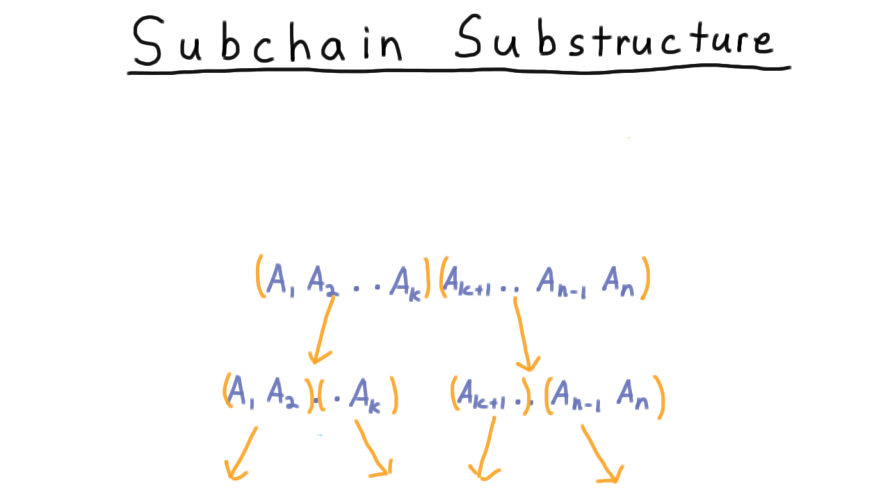
Recursive split strategy: choose a split point \(k\) and solve each half.

Naive recursion recomputes overlapping subproblems — DP avoids this.

Recurrence

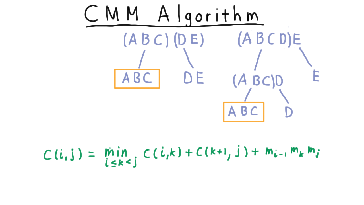
Let \(C(i, j)\) = minimum cost of multiplying matrices \(A_i\) through \(A_j\), where matrix \(A_i\) has dimensions \(m_{i-1} \times m_i\).

\[C(i, j) = \min_{i \leq k < j} \bigl\{ C(i,\, k) + C(k+1,\, j) + m_{i-1} \cdot m_k \cdot m_j \bigr\}\]

Base case:

\[C(i, i) = 0\]

The term \(m_{i-1} \cdot m_k \cdot m_j\) is the cost of multiplying the two resulting subchain matrices together.

Algorithm

Fill an \(n \times n\) table along diagonals from the main diagonal toward the upper-right corner. Each entry \(C(i,j)\) depends only on entries strictly below (smaller subchains).

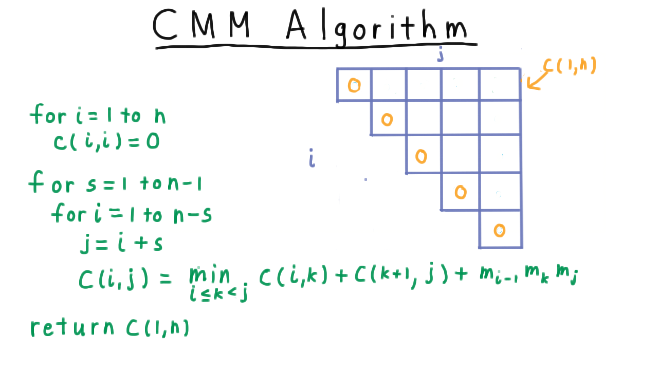
Diagonal fill order — entries depend on cells below and to the left.

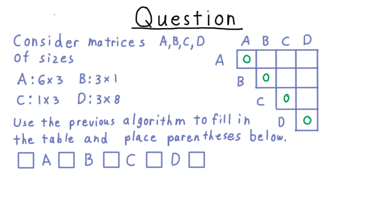
Quiz: Compute the optimal parenthesization cost for matrices \(A, B, C, D\).

Record the split point \(k\) that achieves each minimum to reconstruct the parenthesization.

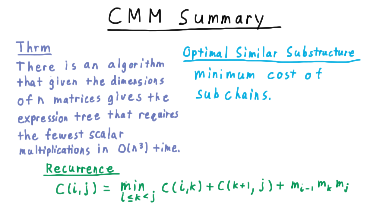
Summary: \(O(n^2)\) subproblems, \(O(n)\) work each → \(O(n^3)\) total.

Time complexity: \(O(n^3)\)

---

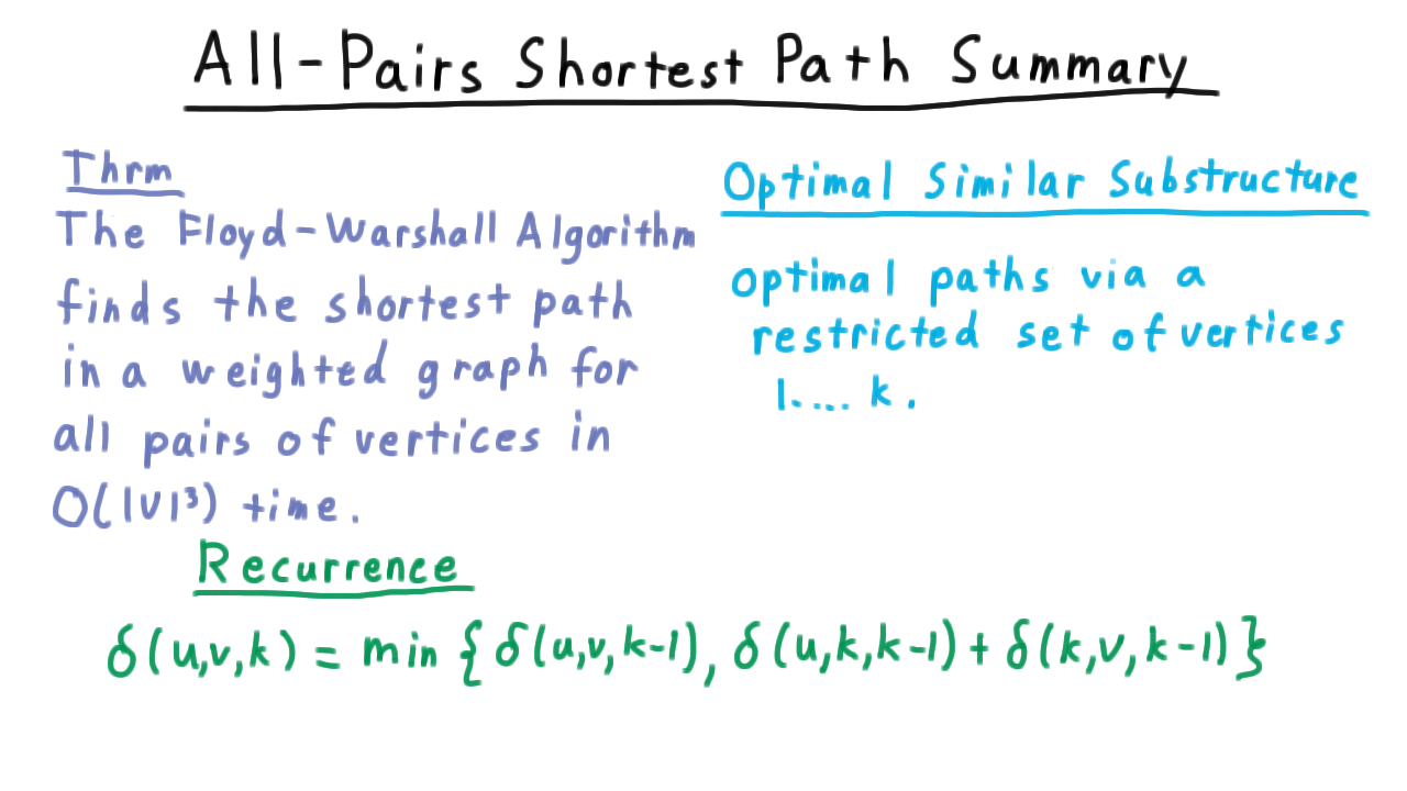
Problem 3: All-Pairs Shortest Paths (Floyd-Warshall)

Goal: Find the shortest-path weight \(\delta(u, v)\) between every pair of vertices in a weighted directed graph.

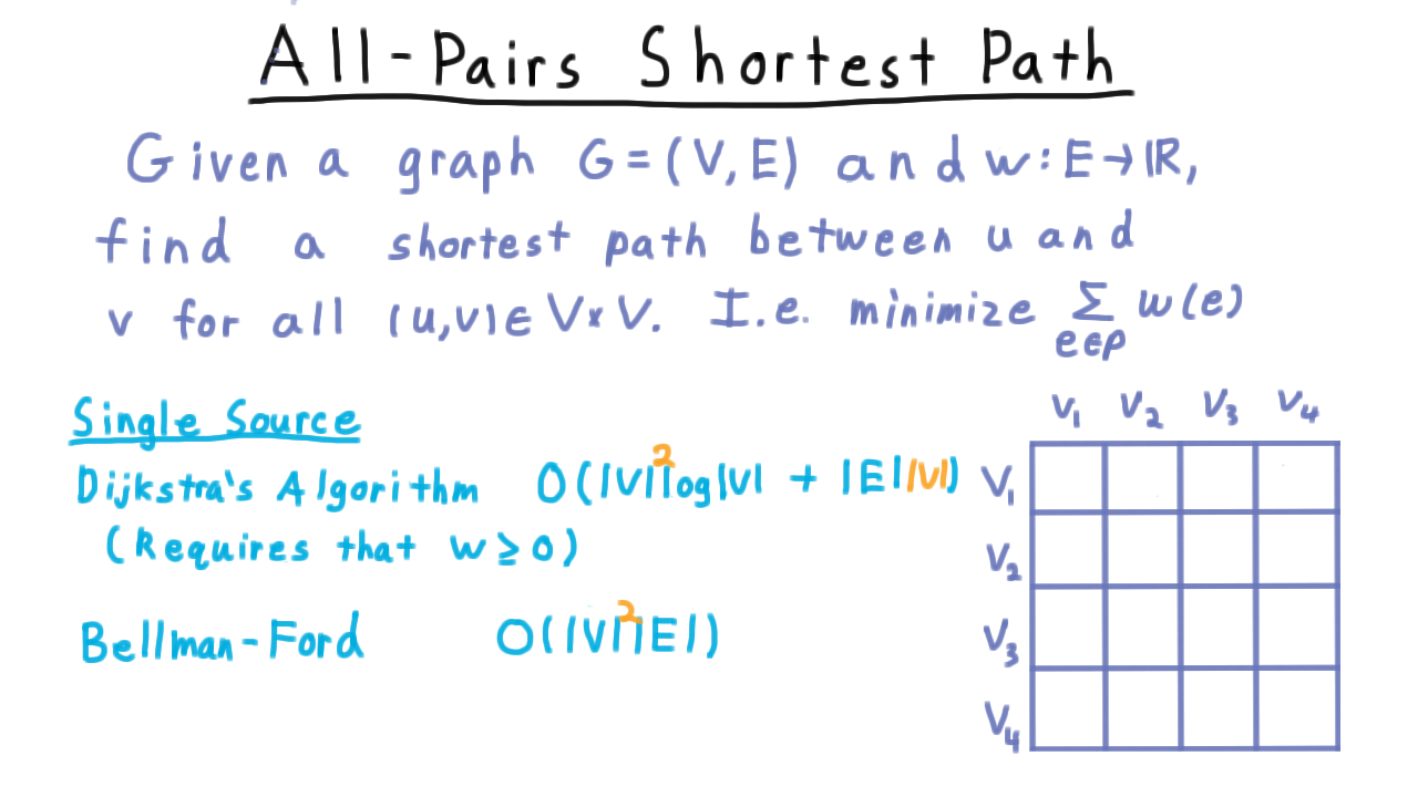
Running a single-source algorithm from every vertex costs \(O(V \cdot E \log V)\) with Dijkstra — Floyd-Warshall achieves \(O(V^3)\).

Optimal Substructure

Subpaths of shortest paths are themselves shortest paths (cut-and-paste argument).

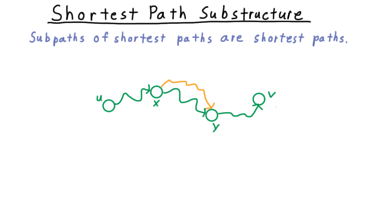
If a subpath were not optimal, replacing it would yield a shorter overall path — contradiction.

The naive approach indexes paths by number of edges, leading to a matrix-multiplication formulation.

Matrix-multiplication approach to all-pairs shortest paths (slower alternative).

Floyd-Warshall instead indexes by the set of allowed intermediate vertices, eliminating circular dependencies.

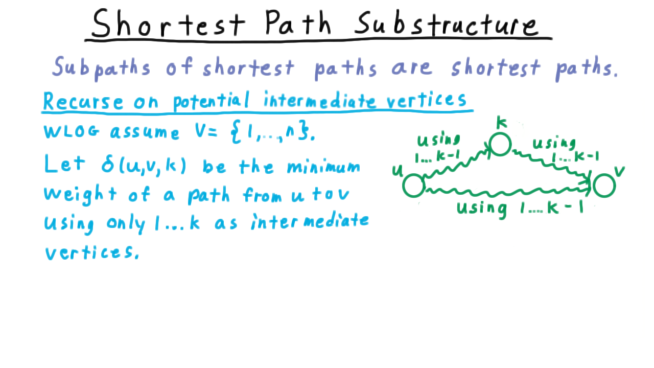
Floyd-Warshall recurrence: restrict intermediate vertices to \(\{1, \ldots, k\}\).

Recurrence

Let \(\delta(u, v, k)\) = minimum-weight path from \(u\) to \(v\) using only vertices \(\{1, \ldots, k\}\) as intermediates.

\[\begin{split}\delta(u, v, k) = \min \begin{cases} \delta(u,\, v,\, k-1) & \text{(don't use vertex } k \text{)} \\ \delta(u,\, k,\, k-1) + \delta(k,\, v,\, k-1) & \text{(route through vertex } k \text{)} \end{cases}\end{split}\]

Base case:

\[\begin{split}\delta(u, v, 0) = \begin{cases} w(u, v) & \text{if edge } (u,v) \text{ exists} \\ \infty & \text{otherwise} \end{cases}\end{split}\]

Algorithm

Initialize a \(V \times V\) distance matrix with direct edge weights (and \(\infty\) for missing edges). For each \(k = 1\) to \(V\), update every pair \((u, v)\):

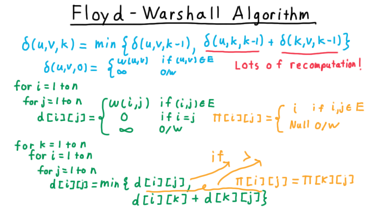
Floyd-Warshall pseudocode — three nested loops, updating in-place.

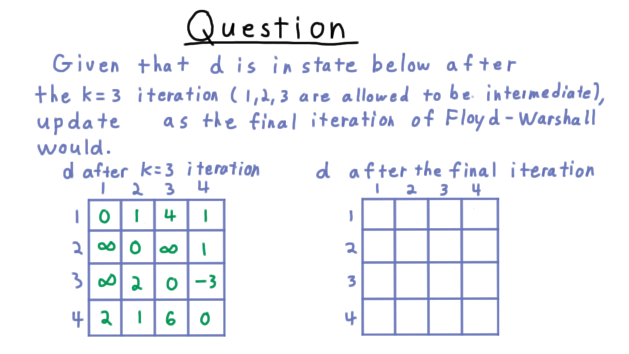
Quiz: Complete the distance matrix after the \(k = 4\) iteration.

Maintain a predecessor matrix alongside the distance matrix to reconstruct actual paths.

Summary: \(O(V^3)\) time, \(O(V^2)\) space.

Time complexity: \(O(V^3)\)

Transitive Closure

The same structure computes the transitive closure of a relation — whether a path exists rather than its weight — by replacing weights with booleans:

\[t(u, v, k) = t(u,\, v,\, k-1) \;\lor\; \bigl(t(u,\, k,\, k-1) \land t(k,\, v,\, k-1)\bigr)\]

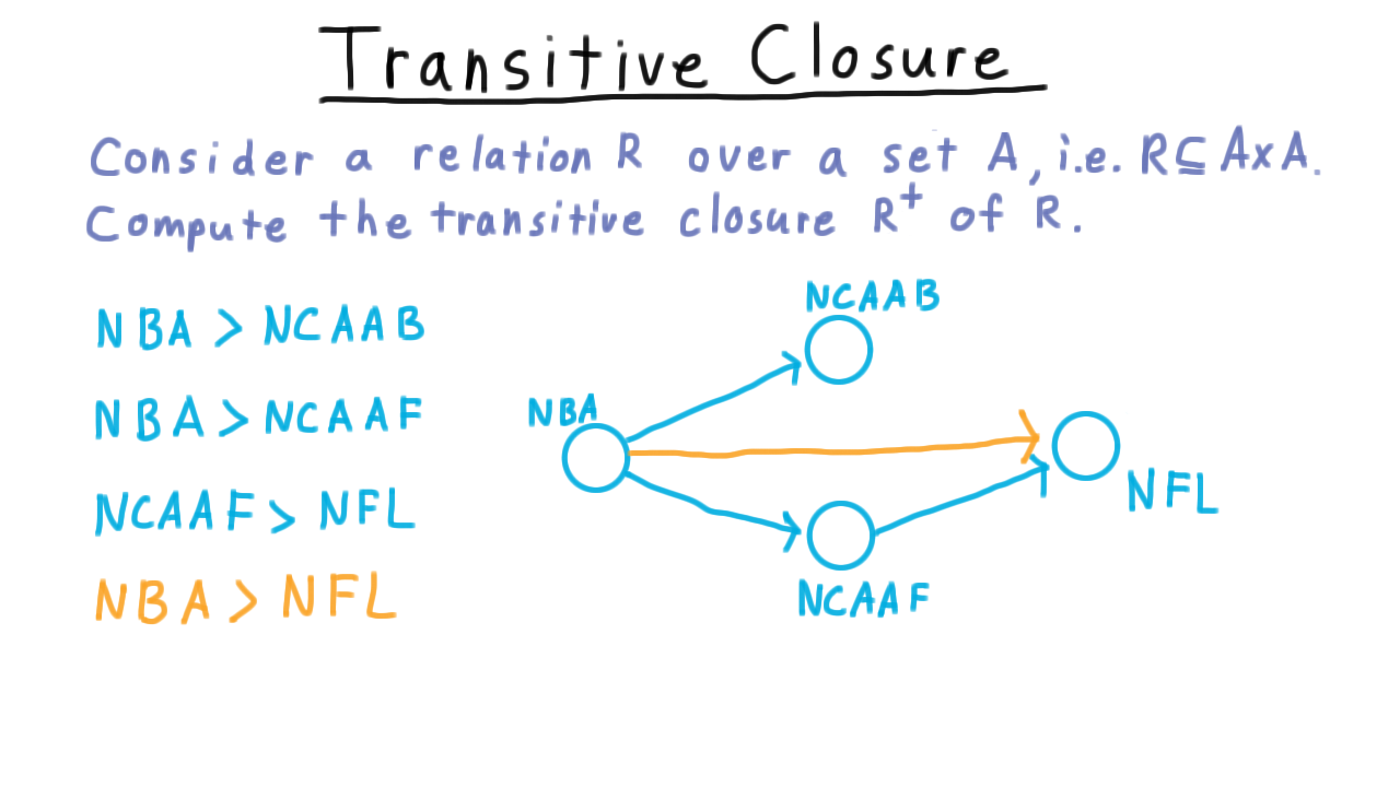
Directed graph example: does player \(u\) (transitively) prefer sport \(v\)?

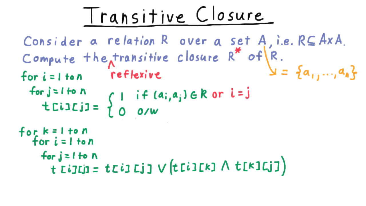
Boolean Floyd-Warshall computes the full transitive closure in \(O(V^3)\).

---

DP Design Recipe

1. Identify substructure — express the optimum recursively in terms of smaller subproblems.

2. Write the recurrence — define \(OPT(i, \ldots)\) and how it decomposes.

3. State base cases — trivial instances with known answers.

4. Choose fill order — arrange computation so every dependency is already solved.

5. Implement iteratively — build a table; avoid recursion to prevent recomputation.

6. Reconstruct solution — trace back through stored decisions.

---

Limitations

DP does not guarantee polynomial time for all recursively-defined problems. For example, SAT has a valid recursive formulation (try \(x_i = \text{true}\) / \(\text{false}\) and recurse), yet no polynomial DP is known — subproblem overlap is insufficient for exploitation unless \(P = NP\).

---

Complexity Summary

Problem	Subproblems	Time
Sequence Alignment	\(O(mn)\)	\(O(mn)\)
Chain Matrix Multiplication	\(O(n^2)\)	\(O(n^3)\)
All-Pairs Shortest Paths	\(O(V^2)\)	\(O(V^3)\)
Transitive Closure	\(O(V^2)\)	\(O(V^3)\)

---

Key Recurrences

Sequence alignment:

\[c(i, j) = \min\bigl\{\, c(i-1,j-1) + \alpha(X_i, Y_j),\quad c(i-1,j)+1,\quad c(i,j-1)+1 \,\bigr\}\]

Chain matrix multiplication:

\[C(i, j) = \min_{i \leq k < j}\bigl\{\, C(i,k) + C(k+1,j) + m_{i-1} m_k m_j \,\bigr\}\]

Floyd-Warshall:

\[\delta(u,v,k) = \min\bigl\{\, \delta(u,v,k-1),\quad \delta(u,k,k-1) + \delta(k,v,k-1) \,\bigr\}\]